Geographical distribution and coverage of signature types
import xarray
import rioxarray
import numpy
import geopandas
import pandas
import contextily
import matplotlib
import matplotlib.pyplot as plt
import urbangrammar_graphics as ugg
import dask.dataframe as dd
from shapely.geometry import Point
from matplotlib_scalebar.scalebar import ScaleBar

# import squarify
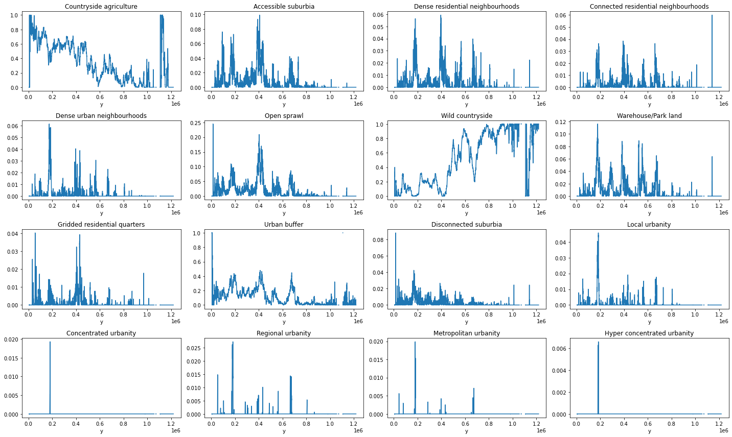
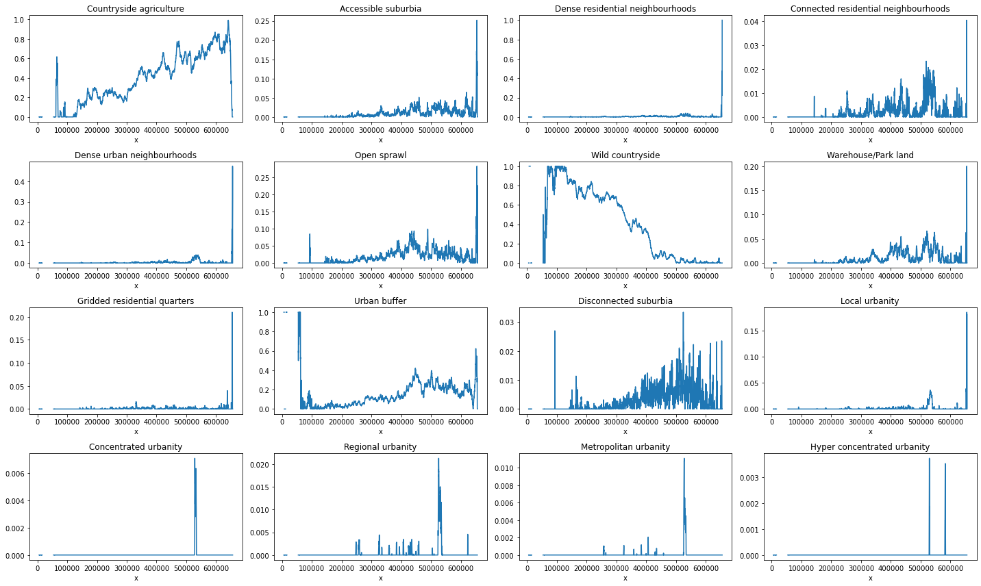
Geographical distribution along N-S and E-W axes
signatures = rioxarray.open_rasterio("../../urbangrammar_samba/spatial_signatures/signatures/signatures_raster.tif")
unique = numpy.unique(signatures[0])
unique = unique[~numpy.isnan(unique)]
outliers = [93, 96, 97, 98]
unique = unique[~numpy.isin(unique, outliers)]
total_by_row = signatures[0].count("x")
total_by_col = signatures[0].count("y")
types = {
    0: "Countryside agriculture",
    10: "Accessible suburbia",
    30: "Open sprawl",
    40: "Wild countryside",
    50: "Warehouse/Park land",
    60: "Gridded residential quarters",
    70: "Urban buffer",
    80: "Disconnected suburbia",
    20: "Dense residential neighbourhoods",
    21: "Connected residential neighbourhoods",
    22: "Dense urban neighbourhoods",
    90: "Local urbanity",
    91: "Concentrated urbanity",
    92: "Regional urbanity",
    94: "Metropolitan urbanity",
    95: "Hyper concentrated urbanity",
}
proportion_by_lat = {}
proportion_by_lon = {}

for label in unique:
    proportion_by_lat[types[label]] = ((signatures[0] == label).sum("x") / total_by_row)
    proportion_by_lon[types[label]] = ((signatures[0] == label).sum("y") / total_by_col)
fig, axs = plt.subplots(4, 4, figsize=(20, 12))

for label, ax in zip(proportion_by_lat, axs.flatten()):
    proportion_by_lat[label].plot(ax=ax)
    ax.set_title(label)
plt.tight_layout()
fig, axs = plt.subplots(4, 4, figsize=(20, 12))

for label, ax in zip(proportion_by_lon, axs.flatten()):
    proportion_by_lon[label].plot(ax=ax)
    ax.set_title(label)
plt.tight_layout()
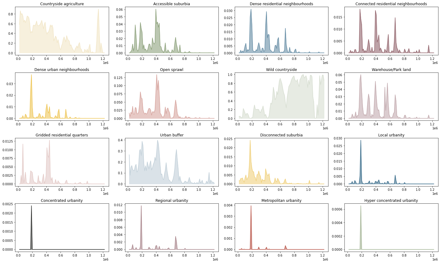
Resample and assign color
types = {
    "0_0": "Countryside agriculture",
    "1_0": "Accessible suburbia",
    "3_0": "Open sprawl",
    "4_0": "Wild countryside",
    "5_0": "Warehouse/Park land",
    "6_0": "Gridded residential quarters",
    "7_0": "Urban buffer",
    "8_0": "Disconnected suburbia",
    "2_0": "Dense residential neighbourhoods",
    "2_1": "Connected residential neighbourhoods",
    "2_2": "Dense urban neighbourhoods",
    "9_0": "Local urbanity",
    "9_1": "Concentrated urbanity",
    "9_2": "Regional urbanity",
    "9_4": "Metropolitan urbanity",
    "9_5": "Hyper concentrated urbanity",
}
cmap = ugg.get_colormap(20, randomize=False)
cols = cmap.colors

symbology = {'0_0': cols[16],
             '1_0': cols[15],
             '3_0': cols[9],
             '4_0': cols[12],
             '5_0': cols[21],
             '6_0': cols[8],
             '7_0': cols[4],
             '8_0': cols[18],
             '2_0': cols[6],
             '2_1': cols[23],
             '2_2': cols[19],
             '9_0': cols[7],
             '9_1': cols[3],
             '9_2': cols[22],
             '9_4': cols[11],
             '9_5': cols[14],
            }
symbology = {types[k]:v for k, v in symbology.items()}
sig = "Countryside agriculture"
x = proportion_by_lat[sig].fillna(0).values
y = proportion_by_lat[sig].y.values
lat = numpy.linspace(proportion_by_lat[sig].y.max(), proportion_by_lat[sig].y.min(), 100, endpoint=False)
f = []
for i, v in enumerate(lat):
    try:
        mask = (v > y) & (y > lat[i+1])
    except:
        mask = v > y
    f.append(x[mask].mean())
fig, axs = plt.subplots(4, 4, figsize=(20, 12))

for sig, ax in zip(proportion_by_lat, axs.flatten()):
    x = proportion_by_lat[sig].fillna(0).values
    y = proportion_by_lat[sig].y.values
    lat = np.linspace(proportion_by_lat[sig].y.max(), proportion_by_lat[sig].y.min(), 100, endpoint=False)
    f = []
    for i, v in enumerate(lat):
        try:
            mask = (v > y) & (y > lat[i+1])
        except:
            mask = v > y
        f.append(x[mask].mean())
    ax.plot(lat, f, color=symbology[sig])
    ax.fill_between(lat, 0, f, color=symbology[sig], alpha=.6)
    ax.set_title(sig)
plt.tight_layout()
plt.savefig("figs/by_lat.pdf")
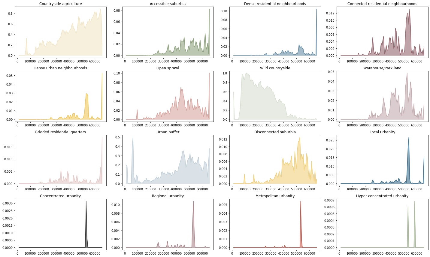
fig, axs = plt.subplots(4, 4, figsize=(20, 12))

for sig, ax in zip(proportion_by_lat, axs.flatten()):
    x = proportion_by_lon[sig].fillna(0).values
    y = proportion_by_lon[sig].x.values
    lat = np.linspace(proportion_by_lon[sig].x.max(), proportion_by_lon[sig].x.min(), 100, endpoint=False)
    f = []
    for i, v in enumerate(lat):
        try:
            mask = (v > y) & (y > lat[i+1])
        except:
            mask = v > y
        f.append(x[mask].mean())
    ax.plot(lat, f, color=symbology[sig])
    ax.fill_between(lat, 0, f, color=symbology[sig], alpha=.6)
    ax.set_title(sig)
plt.tight_layout()
plt.savefig("figs/by_lon.pdf")
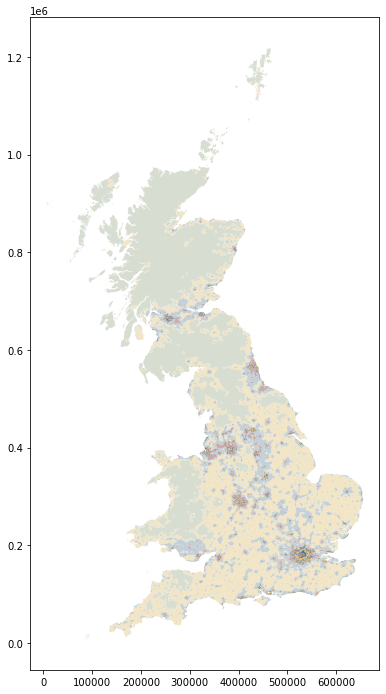
Plot map
signatures = geopandas.read_parquet("../../urbangrammar_samba/spatial_signatures/signatures/signatures_combined_levels_simplified.pq")
signatures["signature_type"] = signatures["signature_type"].map(types)
signatures = signatures.dropna()
signatures.plot(figsize=(12, 12), color=signatures["signature_type"].map(symbology))
plt.savefig("figs/signature_map.png", dpi=300)
Coverage
signatures["area"] = signatures.area
types_sum = signatures[["area", "signature_type"]].groupby("signature_type").sum()
types_sum
| area | |
|---|---|
| signature_type | |
| Accessible suburbia | 2.244586e+09 |
| Concentrated urbanity | 7.883216e+06 |
| Connected residential neighbourhoods | 5.654034e+08 |
| Countryside agriculture | 9.385615e+10 |
| Dense residential neighbourhoods | 9.572622e+08 |
| Dense urban neighbourhoods | 5.706291e+08 |
| Disconnected suburbia | 7.089617e+08 |
| Gridded residential quarters | 2.612541e+08 |
| Hyper concentrated urbanity | 2.293596e+06 |
| Local urbanity | 2.311573e+08 |
| Metropolitan urbanity | 1.658261e+07 |
| Open sprawl | 5.081598e+09 |
| Regional urbanity | 7.643967e+07 |
| Urban buffer | 3.158887e+10 |
| Warehouse/Park land | 2.462472e+09 |
| Wild countryside | 9.130631e+10 |
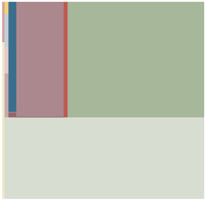
fig, ax = plt.subplots(figsize=(12, 12))
squarify.plot(sizes=types_sum.area, pad=False, ax=ax, color=list(symbology.values()))
ax.axis('off')
(0.0, 100.0, 0.0, 100.0)
types_sum["color"] = [symbology[c] for c in types_sum.index]
types_sum
| area | color | |
|---|---|---|
| signature_type | ||
| Accessible suburbia | 2.244586e+09 | (0.5625, 0.640625, 0.4921875) |
| Concentrated urbanity | 7.883216e+06 | (0.19921875, 0.203125, 0.1953125) |
| Connected residential neighbourhoods | 5.654034e+08 | (0.58203125, 0.3984375, 0.4296875) |
| Countryside agriculture | 9.385615e+10 | (0.9475259828670731, 0.9021947232500418, 0.782... |
| Dense residential neighbourhoods | 9.572622e+08 | (0.405436326872467, 0.5568241504426759, 0.6493... |
| Dense urban neighbourhoods | 5.706291e+08 | (0.9375, 0.78125, 0.34375) |
| Disconnected suburbia | 7.089617e+08 | (0.9408069995844273, 0.8211427621191237, 0.488... |
| Gridded residential quarters | 2.612541e+08 | (0.8956450438496885, 0.7949476416458632, 0.782... |
| Hyper concentrated urbanity | 2.293596e+06 | (0.6550082934095629, 0.716277287243688, 0.6001... |
| Local urbanity | 2.311573e+08 | (0.23046875, 0.4296875, 0.55078125) |
| Metropolitan urbanity | 1.658261e+07 | (0.73828125, 0.35546875, 0.30859375) |
| Open sprawl | 5.081598e+09 | (0.8429158144969133, 0.6476876988954169, 0.623... |
| Regional urbanity | 7.643967e+07 | (0.6718003015294096, 0.5329645862558573, 0.556... |
| Urban buffer | 3.158887e+10 | (0.7609260068673207, 0.8151335354690646, 0.849... |
| Warehouse/Park land | 2.462472e+09 | (0.7629942586386511, 0.6696270230872043, 0.685... |
| Wild countryside | 9.130631e+10 | (0.8429616514480401, 0.8699835216435621, 0.819... |
types_sum = types_sum.sort_values("area", ascending=False)
ax = types_sum.area.plot.bar(color=types_sum.color)
ax.set_yscale("log")
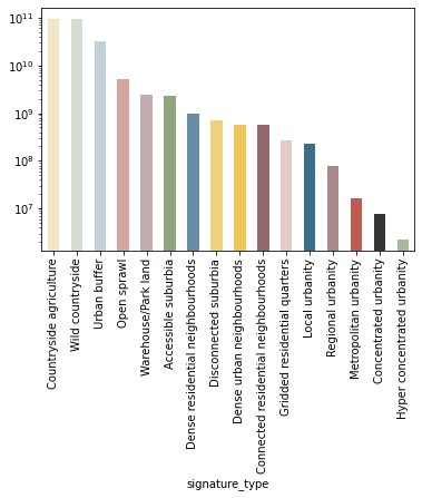
types_sum.sort_values("area", ascending=False).index
Index(['Countryside agriculture', 'Wild countryside', 'Urban buffer',
       'Open sprawl', 'Warehouse/Park land', 'Accessible suburbia',
       'Dense residential neighbourhoods', 'Disconnected suburbia',
       'Dense urban neighbourhoods', 'Connected residential neighbourhoods',
       'Gridded residential quarters', 'Local urbanity', 'Regional urbanity',
       'Metropolitan urbanity', 'Concentrated urbanity',
       'Hyper concentrated urbanity'],
      dtype='object', name='signature_type')
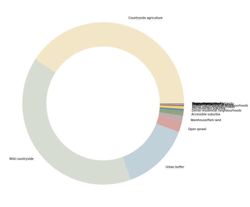
fig, ax = plt.subplots(figsize=(12, 12))
types_sum.area.plot.pie(colors=types_sum.color, labels=types_sum.index, ax=ax, normalize=True)
ax.axis("off")
ax.add_artist(plt.Circle((0,0), .7, color="w"))
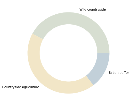
countryside = types_sum.loc[["Wild countryside", "Countryside agriculture", "Urban buffer"]]

fig, ax = plt.subplots(figsize=(6, 6))
countryside.area.plot.pie(colors=countryside.color, labels=countryside.index, ax=ax, normalize=True)
ax.axis("off")
ax.add_artist(plt.Circle((0,0), .7, color="w"))
plt.savefig("fig/cov_countryside.pdf")
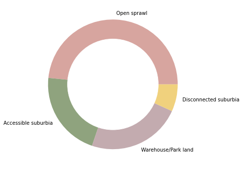
periphery = types_sum.loc[["Open sprawl", "Accessible suburbia", "Warehouse/Park land", "Disconnected suburbia"]]

fig, ax = plt.subplots(figsize=(6, 6))
periphery.area.plot.pie(colors=periphery.color, labels=periphery.index, ax=ax, normalize=True)
ax.axis("off")
ax.add_artist(plt.Circle((0,0), .7, color="w"))
plt.savefig("fig/cov_periphery.pdf")
centres = types_sum.loc[[c for c in types_sum.index if c not in periphery.index.union(countryside.index)]]

fig, ax = plt.subplots(figsize=(6, 6))
centres.area.plot.pie(colors=centres.color, labels=None, ax=ax, normalize=True)
ax.axis("off")
ax.add_artist(plt.Circle((0,0), .7, color="w"))
ax.text(0.48081342961609136, 0.9893525387347082, 'Dense residential neighbourhoods')
ax.text(-2.268978614659921, 0.2593929864120394, 'Dense urban neighbourhoods')
ax.text(-1.994807053876901, -0.9748996927056968, 'Connected residential neighbourhoods')
ax.text(0.51211504741639, -0.9735184529374411, 'Gridded residential quarters')
ax.text(0.959363500900176, -0.538165098404345, 'Local urbanity')
ax.text(1.087344357909379, -0.16637982847280644, 'Regional urbanity')
ax.text(1.098975902527664, -0.08745488029177633, 'Metropolitan urbanity')
ax.text(1.0998832541521082, -0.01602583026770399, 'Concentrated urbanity')
ax.text(1.09999605164628, 0.045, 'Hyper concentrated urbanity')
plt.savefig("fig/cov_centres.pdf")

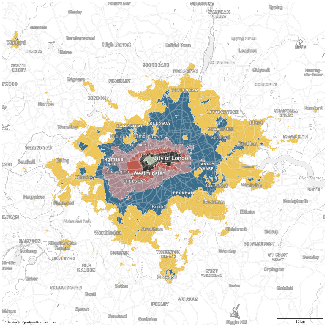
london = geopandas.GeoSeries([Point(-0.10875602230396436, 51.50933674406198)], crs=4326).to_crs(27700).buffer(35000).total_bounds
df = signatures.cx[london[0]:london[2], london[1]:london[3]].to_crs(3857)
centre_types = ['Hyper concentrated urbanity', 'Concentrated urbanity', 'Metropolitan urbanity', 'Regional urbanity', 'Local urbanity', 'Dense urban neighbourhoods']

df_centres = df.loc[df.signature_type.isin(centre_types)]
df_out = df.loc[~df.signature_type.isin(centre_types)]
ax = df_centres.plot(color=df_centres['signature_type'].map(symbology), figsize=(20, 20), zorder=1, linewidth=.3, edgecolor='w', alpha=1)
# df_out.plot(ax=ax, color=df_out['signature_type'].map(symbology), zorder=1, linewidth=.3, edgecolor='w', alpha=.5)

london = geopandas.GeoSeries([Point(-0.10875602230396436, 51.50933674406198)], crs=4326).to_crs(3857).buffer(35000).total_bounds
ax.set_xlim(london[0], london[2])
ax.set_ylim(london[1], london[3])

contextily.add_basemap(ax, crs=df_centres.crs, source=ugg.get_tiles('roads', token), zorder=2, alpha=.3)
contextily.add_basemap(ax, crs=df_centres.crs, source=ugg.get_tiles('labels', token), zorder=3, alpha=1)
contextily.add_basemap(ax, crs=df_centres.crs, source=ugg.get_tiles('background', token), zorder=-1, alpha=1)
ax.set_axis_off()

scalebar = ScaleBar(dx=1,
                    color=ugg.COLORS[0],
                    location='lower right',
                    height_fraction=0.002,
                    pad=.5,
                    frameon=False,
                    )
ax.add_artist(scalebar)

# ugg.north_arrow(plt.gcf(), ax, 0, size=.05, linewidth=1, color=ugg.COLORS[0], loc="upper left", pad=.002, alpha=.9)

# custom_points = [Line2D([0], [0], marker="o", linestyle="none", markersize=10, color=color) for color in symbology.values()]
# leg_points = ax.legend(custom_points, symbology.keys(), bbox_to_anchor=(1.05, 1), loc='upper left', frameon=True)
# ax.add_artist(leg_points)
plt.savefig("figs/signatures_london_centres.png", dpi=72, bbox_inches="tight")
Count of tessellation cells by type
import geopandas
import dask_geopandas
import pandas
tess = dask_geopandas.read_parquet(f"../../urbangrammar_samba/spatial_signatures/tessellation/tess_*.pq")
labels_l1 = pandas.read_parquet("../../urbangrammar_samba/spatial_signatures/clustering_data/KMeans10GB.pq")
labels_l2_9 = pandas.read_parquet("../../urbangrammar_samba/spatial_signatures/clustering_data/clustergram_cl9_labels.pq")
labels_l2_2 = pandas.read_parquet("../../urbangrammar_samba/spatial_signatures/clustering_data/subclustering_cluster2_k3.pq")
labels = labels_l1.copy()
labels.loc[labels.kmeans10gb == 9, 'kmeans10gb'] = labels_l2_9['9'].values + 90
labels.loc[labels.kmeans10gb == 2, 'kmeans10gb'] = labels_l2_2['subclustering_cluster2_k3'].values + 20

outliers = [98, 93, 96, 97]
mask = ~labels.kmeans10gb.isin(outliers)
labels[mask]["kmeans10gb"].value_counts().to_csv("../../urbangrammar_samba/spatial_signatures/esda/counts.csv")
labels[mask]["kmeans10gb"].value_counts()
7     3686554
0     3022385
3     2561211
1     1962830
5      707211
4      595902
8      564318
20     502835
21     374090
22     238639
6      209959
90      86380
92      21760
94       3739
91       1390
95        264
Name: kmeans10gb, dtype: int64
signatures = geopandas.read_parquet("../../urbangrammar_samba/spatial_signatures/signatures/signatures_combined_levels_simplified.pq")

signatures["area"] = signatures.area
types_sum = signatures[["area", "signature_type"]].groupby("signature_type").sum()
counts = pandas.read_csv("../../urbangrammar_samba/spatial_signatures/esda/counts.csv", index_col=0
                        )
types_sum
| area | |
|---|---|
| signature_type | |
| 0_0 | 9.385615e+10 |
| 1_0 | 2.244586e+09 |
| 2_0 | 9.572622e+08 |
| 2_1 | 5.654034e+08 |
| 2_2 | 5.706291e+08 |
| 3_0 | 5.081598e+09 |
| 4_0 | 9.130631e+10 |
| 5_0 | 2.462472e+09 |
| 6_0 | 2.612541e+08 |
| 7_0 | 3.158887e+10 |
| 8_0 | 7.089617e+08 |
| 9_0 | 2.311573e+08 |
| 9_1 | 7.883216e+06 |
| 9_2 | 7.643967e+07 |
| 9_3 | 1.376262e+05 |
| 9_4 | 1.658261e+07 |
| 9_5 | 2.293596e+06 |
| 9_6 | 4.207900e+05 |
| 9_7 | 3.958330e+05 |
| 9_8 | 4.091500e+05 |
idx = []
for i in counts.index:
    i = str(i)
    if len(i) == 1:
        idx.append(i + "_0")
    else:
        idx.append(i[0] + "_" + i[1])
counts
| kmeans10gb | |
|---|---|
| 7 | 3686554 |
| 0 | 3022385 |
| 3 | 2561211 |
| 1 | 1962830 |
| 5 | 707211 |
| 4 | 595902 |
| 8 | 564318 |
| 20 | 502835 |
| 21 | 374090 |
| 22 | 238639 |
| 6 | 209959 |
| 90 | 86380 |
| 92 | 21760 |
| 94 | 3739 |
| 91 | 1390 |
| 95 | 264 |
counts.index = idx
types_sum['counts'] = counts.kmeans10gb
types_sum = types_sum.dropna()
types_sum.index = types_sum.index.map(types)
types_sum["area_perc"] = (types_sum.area / types_sum.area.sum()) * 100
types_sum["count_perc"] = (types_sum.counts / types_sum.counts.sum()) * 100
/tmp/ipykernel_419951/3349044170.py:1: SettingWithCopyWarning:
A value is trying to be set on a copy of a slice from a DataFrame.
Try using .loc[row_indexer,col_indexer] = value instead

See the caveats in the documentation: https://pandas.pydata.org/pandas-docs/stable/user_guide/indexing.html#returning-a-view-versus-a-copy
  types_sum["area_perc"] = (types_sum.area / types_sum.area.sum()) * 100
/tmp/ipykernel_419951/3349044170.py:2: SettingWithCopyWarning:
A value is trying to be set on a copy of a slice from a DataFrame.
Try using .loc[row_indexer,col_indexer] = value instead

See the caveats in the documentation: https://pandas.pydata.org/pandas-docs/stable/user_guide/indexing.html#returning-a-view-versus-a-copy
  types_sum["count_perc"] = (types_sum.counts / types_sum.counts.sum()) * 100
types_sum
| area | counts | area_perc | count_perc | |
|---|---|---|---|---|
| signature_type | ||||
| Countryside agriculture | 9.385615e+10 | 3022385.0 | 40.818050 | 20.787454 |
| Accessible suburbia | 2.244586e+09 | 1962830.0 | 0.976171 | 13.500013 |
| Dense residential neighbourhoods | 9.572622e+08 | 502835.0 | 0.416313 | 3.458414 |
| Connected residential neighbourhoods | 5.654034e+08 | 374090.0 | 0.245894 | 2.572928 |
| Dense urban neighbourhoods | 5.706291e+08 | 238639.0 | 0.248167 | 1.641319 |
| Open sprawl | 5.081598e+09 | 2561211.0 | 2.209988 | 17.615577 |
| Wild countryside | 9.130631e+10 | 595902.0 | 39.709124 | 4.098513 |
| Warehouse/Park land | 2.462472e+09 | 707211.0 | 1.070930 | 4.864078 |
| Gridded residential quarters | 2.612541e+08 | 209959.0 | 0.113619 | 1.444063 |
| Urban buffer | 3.158887e+10 | 3686554.0 | 13.738005 | 25.355496 |
| Disconnected suburbia | 7.089617e+08 | 564318.0 | 0.308328 | 3.881284 |
| Local urbanity | 2.311573e+08 | 86380.0 | 0.100530 | 0.594107 |
| Concentrated urbanity | 7.883216e+06 | 1390.0 | 0.003428 | 0.009560 |
| Regional urbanity | 7.643967e+07 | 21760.0 | 0.033244 | 0.149662 |
| Metropolitan urbanity | 1.658261e+07 | 3739.0 | 0.007212 | 0.025716 |
| Hyper concentrated urbanity | 2.293596e+06 | 264.0 | 0.000997 | 0.001816 |
print(types_sum.round(0).to_latex(float_format="%.0f"))
\begin{tabular}{lrrrr}
\toprule
{} &        area &  counts &  area\_perc &  count\_perc \\
signature\_type                       &             &         &            &             \\
\midrule
Countryside agriculture              & 93856149107 & 3022385 &         41 &          21 \\
Accessible suburbia                  &  2244586111 & 1962830 &          1 &          14 \\
Dense residential neighbourhoods     &   957262179 &  502835 &          0 &           3 \\
Connected residential neighbourhoods &   565403381 &  374090 &          0 &           3 \\
Dense urban neighbourhoods           &   570629053 &  238639 &          0 &           2 \\
Open sprawl                          &  5081598096 & 2561211 &          2 &          18 \\
Wild countryside                     & 91306307616 &  595902 &         40 &           4 \\
Warehouse/Park land                  &  2462472439 &  707211 &          1 &           5 \\
Gridded residential quarters         &   261254080 &  209959 &          0 &           1 \\
Urban buffer                         & 31588874152 & 3686554 &         14 &          25 \\
Disconnected suburbia                &   708961672 &  564318 &          0 &           4 \\
Local urbanity                       &   231157300 &   86380 &          0 &           1 \\
Concentrated urbanity                &     7883216 &    1390 &          0 &           0 \\
Regional urbanity                    &    76439673 &   21760 &          0 &           0 \\
Metropolitan urbanity                &    16582607 &    3739 &          0 &           0 \\
Hyper concentrated urbanity          &     2293596 &     264 &          0 &           0 \\
\bottomrule
\end{tabular}
path = "../../urbangrammar_samba/spatial_signatures/functional/population"
population = dd.read_parquet(path)
types_path = "../../urbangrammar_samba/spatial_signatures/signatures/signatures_combined_tessellation"
sig_types = dd.read_parquet(types_path, columns=['hindex', 'signature_type'])
sig_types.head()
| hindex | signature_type | |
|---|---|---|
| 0 | c000e109777t0000 | 6 |
| 1 | c000e109777t0001 | 6 |
| 2 | c000e109777t0002 | 6 |
| 3 | c000e109777t0003 | 6 |
| 4 | c000e109777t0004 | 6 |
combined = population.merge(sig_types, on='hindex', how="left")
combined
Dask DataFrame Structure:
| hindex | population | signature_type | |
|---|---|---|---|
| npartitions=103 | |||
| object | float64 | int32 | |
| ... | ... | ... | |
| ... | ... | ... | ... |
| ... | ... | ... | |
| ... | ... | ... |
Dask Name: hash-join, 1549 tasks
summary = combined.groupby('signature_type').agg({"population": sum, "hindex": "count"})
summary = summary.compute()
Check the sum, should be above 67 mio.
summary.population.sum()
67140883.00504927
summary = summary.rename(columns={
    "hindex": "count",
})
types = {
    0: "Countryside agriculture",
    1: "Accessible suburbia",
    3: "Open sprawl",
    4: "Wild countryside",
    5: "Warehouse/Park land",
    6: "Gridded residential quarters",
    7: "Urban buffer",
    8: "Disconnected suburbia",
    20: "Dense residential neighbourhoods",
    21: "Connected residential neighbourhoods",
    22: "Dense urban neighbourhoods",
    90: "Local urbanity",
    91: "Concentrated urbanity",
    92: "Regional urbanity",
    94: "Metropolitan urbanity",
    95: "Hyper concentrated urbanity",
    93: "outlier",
    96: "outlier",
    97: "outlier",
    98: "outlier",
}

summary.index = summary.index.map(types)
summary = summary.drop('outlier')
types_sum['population'] = summary['population']
types_sum["population_perc"] = (types_sum.population / types_sum.population.sum()) * 100
/tmp/ipykernel_419951/1263051370.py:1: SettingWithCopyWarning:
A value is trying to be set on a copy of a slice from a DataFrame.
Try using .loc[row_indexer,col_indexer] = value instead

See the caveats in the documentation: https://pandas.pydata.org/pandas-docs/stable/user_guide/indexing.html#returning-a-view-versus-a-copy
  types_sum['population'] = summary['population']
/tmp/ipykernel_419951/1263051370.py:2: SettingWithCopyWarning:
A value is trying to be set on a copy of a slice from a DataFrame.
Try using .loc[row_indexer,col_indexer] = value instead

See the caveats in the documentation: https://pandas.pydata.org/pandas-docs/stable/user_guide/indexing.html#returning-a-view-versus-a-copy
  types_sum["population_perc"] = (types_sum.population / types_sum.population.sum()) * 100
types_sum
| area | counts | area_perc | count_perc | population | population_perc | |
|---|---|---|---|---|---|---|
| signature_type | ||||||
| Countryside agriculture | 9.385615e+10 | 3022385.0 | 40.818050 | 20.787454 | 5.765794e+06 | 8.587620 |
| Accessible suburbia | 2.244586e+09 | 1962830.0 | 0.976171 | 13.500013 | 8.848915e+06 | 13.179644 |
| Dense residential neighbourhoods | 9.572622e+08 | 502835.0 | 0.416313 | 3.458414 | 5.016013e+06 | 7.470889 |
| Connected residential neighbourhoods | 5.654034e+08 | 374090.0 | 0.245894 | 2.572928 | 3.200903e+06 | 4.767450 |
| Dense urban neighbourhoods | 5.706291e+08 | 238639.0 | 0.248167 | 1.641319 | 4.160981e+06 | 6.197399 |
| Open sprawl | 5.081598e+09 | 2561211.0 | 2.209988 | 17.615577 | 1.291983e+07 | 19.242892 |
| Wild countryside | 9.130631e+10 | 595902.0 | 39.709124 | 4.098513 | 7.738578e+05 | 1.152590 |
| Warehouse/Park land | 2.462472e+09 | 707211.0 | 1.070930 | 4.864078 | 4.885898e+06 | 7.277095 |
| Gridded residential quarters | 2.612541e+08 | 209959.0 | 0.113619 | 1.444063 | 1.622579e+06 | 2.416682 |
| Urban buffer | 3.158887e+10 | 3686554.0 | 13.738005 | 25.355496 | 1.262026e+07 | 18.796710 |
| Disconnected suburbia | 7.089617e+08 | 564318.0 | 0.308328 | 3.881284 | 3.695715e+06 | 5.504427 |
| Local urbanity | 2.311573e+08 | 86380.0 | 0.100530 | 0.594107 | 2.481154e+06 | 3.695450 |
| Concentrated urbanity | 7.883216e+06 | 1390.0 | 0.003428 | 0.009560 | 4.979667e+04 | 0.074168 |
| Regional urbanity | 7.643967e+07 | 21760.0 | 0.033244 | 0.149662 | 9.265150e+05 | 1.379959 |
| Metropolitan urbanity | 1.658261e+07 | 3739.0 | 0.007212 | 0.025716 | 1.626733e+05 | 0.242287 |
| Hyper concentrated urbanity | 2.293596e+06 | 264.0 | 0.000997 | 0.001816 | 9.895050e+03 | 0.014738 |
types_sum.to_csv("summary.csv")
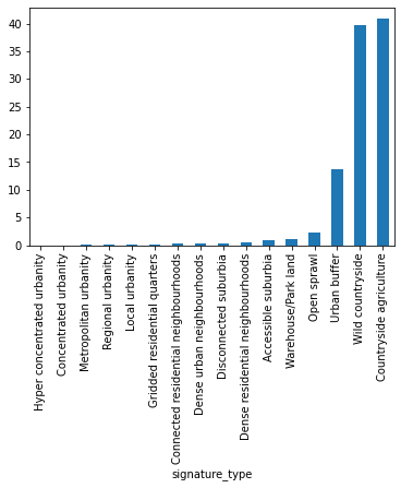
types_sum['population_perc'].sort_values().plot.bar()
<AxesSubplot:xlabel='signature_type'>
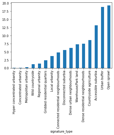
types_sum['area_perc'].sort_values().plot.bar()
<AxesSubplot:xlabel='signature_type'>
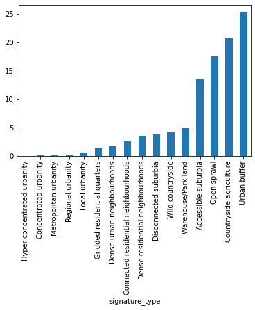
types_sum['count_perc'].sort_values().plot.bar()
<AxesSubplot:xlabel='signature_type'>
types_sum
| area | counts | area_perc | count_perc | population | population_perc | |
|---|---|---|---|---|---|---|
| signature_type | ||||||
| Countryside agriculture | 9.385615e+10 | 3022385.0 | 40.818050 | 20.787454 | 5.765794e+06 | 8.587620 |
| Accessible suburbia | 2.244586e+09 | 1962830.0 | 0.976171 | 13.500013 | 8.848915e+06 | 13.179644 |
| Dense residential neighbourhoods | 9.572622e+08 | 502835.0 | 0.416313 | 3.458414 | 5.016013e+06 | 7.470889 |
| Connected residential neighbourhoods | 5.654034e+08 | 374090.0 | 0.245894 | 2.572928 | 3.200903e+06 | 4.767450 |
| Dense urban neighbourhoods | 5.706291e+08 | 238639.0 | 0.248167 | 1.641319 | 4.160981e+06 | 6.197399 |
| Open sprawl | 5.081598e+09 | 2561211.0 | 2.209988 | 17.615577 | 1.291983e+07 | 19.242892 |
| Wild countryside | 9.130631e+10 | 595902.0 | 39.709124 | 4.098513 | 7.738578e+05 | 1.152590 |
| Warehouse/Park land | 2.462472e+09 | 707211.0 | 1.070930 | 4.864078 | 4.885898e+06 | 7.277095 |
| Gridded residential quarters | 2.612541e+08 | 209959.0 | 0.113619 | 1.444063 | 1.622579e+06 | 2.416682 |
| Urban buffer | 3.158887e+10 | 3686554.0 | 13.738005 | 25.355496 | 1.262026e+07 | 18.796710 |
| Disconnected suburbia | 7.089617e+08 | 564318.0 | 0.308328 | 3.881284 | 3.695715e+06 | 5.504427 |
| Local urbanity | 2.311573e+08 | 86380.0 | 0.100530 | 0.594107 | 2.481154e+06 | 3.695450 |
| Concentrated urbanity | 7.883216e+06 | 1390.0 | 0.003428 | 0.009560 | 4.979667e+04 | 0.074168 |
| Regional urbanity | 7.643967e+07 | 21760.0 | 0.033244 | 0.149662 | 9.265150e+05 | 1.379959 |
| Metropolitan urbanity | 1.658261e+07 | 3739.0 | 0.007212 | 0.025716 | 1.626733e+05 | 0.242287 |
| Hyper concentrated urbanity | 2.293596e+06 | 264.0 | 0.000997 | 0.001816 | 9.895050e+03 | 0.014738 |