Exploration of top-level clusters
This notebook contains intitial exploration of the top-level clusters forming Spatial Signatures in Great Britain.
The notebook looks at the overall similarity of clusters and picks the selection of representative characters to understand what each of the classes is composed of.
import numpy as np
import pandas as pd
import geopandas as gpd
import dask.dataframe
import matplotlib.pyplot as plt
import urbangrammar_graphics as ugg

from matplotlib.lines import Line2D
We need the original data in the same form as was used in the clustering.
%time standardized_form = dask.dataframe.read_parquet("../../urbangrammar_samba/spatial_signatures/clustering_data/form/standardized/").set_index('hindex')
%time stand_fn = dask.dataframe.read_parquet("../../urbangrammar_samba/spatial_signatures/clustering_data/function/standardized/")
%time data = dask.dataframe.multi.concat([standardized_form, stand_fn], axis=1).replace([np.inf, -np.inf], np.nan).fillna(0)
%time data = data.drop(columns=["keep_q1", "keep_q2", "keep_q3"])
%time data = data.compute()
CPU times: user 38.1 s, sys: 32.9 s, total: 1min 11s
Wall time: 1min 44s
CPU times: user 76.8 ms, sys: 461 ms, total: 537 ms
Wall time: 598 ms
CPU times: user 45 ms, sys: 4.3 ms, total: 49.4 ms
Wall time: 43.7 ms
CPU times: user 18.5 ms, sys: 0 ns, total: 18.5 ms
Wall time: 18.4 ms
CPU times: user 2min 40s, sys: 1min 27s, total: 4min 7s
Wall time: 2min 44s
And labels indicating the final cluster for each enclosed tessellation cell.
labels = pd.read_parquet("../../urbangrammar_samba/spatial_signatures/clustering_data/KMeans10GB.pq")
Overall similarity
Similarity of clusters can be represented by hierarchical dendrogram generated using Ward’s agglomerative clustering.
from scipy.cluster import hierarchy
We use cluster centroids (mean value) for the characterisation.
group = data.groupby(labels['kmeans10gb'].values).mean() # cluster centroids
Now we can create hierarchical classification based on cluster centers.
Z = hierarchy.linkage(group, 'ward')
import matplotlib.pyplot as plt
fig, ax = plt.subplots(figsize=(25, 15))
dn = hierarchy.dendrogram(Z, labels=group.index)
plt.grid(True, axis='y', which='both')
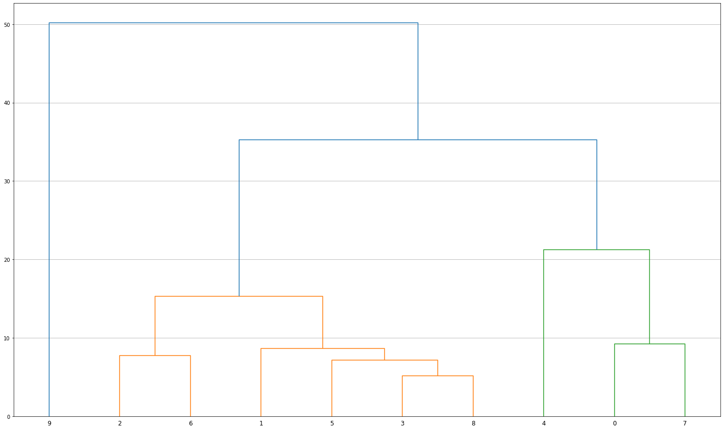
The diagram in the cell above shows that the most dissimilar cluster is the 9 (city centers). The branch on the very right (4, 0, 7) contains predominantly countryside-based signatures. Clusters 2 and 6 form the main bulk of low density development, while the remaining classes (1, 5, 3, 8) cover various industrial, peripheral and fringe locations in cities.
labels['kmeans10gb'].value_counts()
7    3686554
0    3022385
3    2561211
1    1962830
2    1115564
5     707211
4     595902
8     564318
6     209959
9     113644
Name: kmeans10gb, dtype: int64
Classification is relatively balanced with no outlier class in terms of number of observations.
Characterisation
In the section below, we look at some of the characters used within the clustering to characterise the individual categories for a better understandning how they differ.
Let’s see which columns are available.
group.columns.values
array(['sdbAre_q1', 'sdbAre_q2', 'sdbAre_q3', 'sdbPer_q1', 'sdbPer_q2',
       'sdbPer_q3', 'sdbCoA_q1', 'sdbCoA_q2', 'sdbCoA_q3', 'ssbCCo_q1',
       'ssbCCo_q2', 'ssbCCo_q3', 'ssbCor_q1', 'ssbCor_q2', 'ssbCor_q3',
       'ssbSqu_q1', 'ssbSqu_q2', 'ssbSqu_q3', 'ssbERI_q1', 'ssbERI_q2',
       'ssbERI_q3', 'ssbElo_q1', 'ssbElo_q2', 'ssbElo_q3', 'ssbCCM_q1',
       'ssbCCM_q2', 'ssbCCM_q3', 'ssbCCD_q1', 'ssbCCD_q2', 'ssbCCD_q3',
       'stbOri_q1', 'stbOri_q2', 'stbOri_q3', 'sdcLAL_q1', 'sdcLAL_q2',
       'sdcLAL_q3', 'sdcAre_q1', 'sdcAre_q2', 'sdcAre_q3', 'sscCCo_q1',
       'sscCCo_q2', 'sscCCo_q3', 'sscERI_q1', 'sscERI_q2', 'sscERI_q3',
       'stcOri_q1', 'stcOri_q2', 'stcOri_q3', 'sicCAR_q1', 'sicCAR_q2',
       'sicCAR_q3', 'stbCeA_q1', 'stbCeA_q2', 'stbCeA_q3', 'mtbAli_q1',
       'mtbAli_q2', 'mtbAli_q3', 'mtbNDi_q1', 'mtbNDi_q2', 'mtbNDi_q3',
       'mtcWNe_q1', 'mtcWNe_q2', 'mtcWNe_q3', 'mdcAre_q1', 'mdcAre_q2',
       'mdcAre_q3', 'ltcWRE_q1', 'ltcWRE_q2', 'ltcWRE_q3', 'ltbIBD_q1',
       'ltbIBD_q2', 'ltbIBD_q3', 'sdsSPW_q1', 'sdsSPW_q2', 'sdsSPW_q3',
       'sdsSWD_q1', 'sdsSWD_q2', 'sdsSWD_q3', 'sdsSPO_q1', 'sdsSPO_q2',
       'sdsSPO_q3', 'sdsLen_q1', 'sdsLen_q2', 'sdsLen_q3', 'sssLin_q1',
       'sssLin_q2', 'sssLin_q3', 'ldsMSL_q1', 'ldsMSL_q2', 'ldsMSL_q3',
       'mtdDeg_q1', 'mtdDeg_q2', 'mtdDeg_q3', 'lcdMes_q1', 'lcdMes_q2',
       'lcdMes_q3', 'linP3W_q1', 'linP3W_q2', 'linP3W_q3', 'linP4W_q1',
       'linP4W_q2', 'linP4W_q3', 'linPDE_q1', 'linPDE_q2', 'linPDE_q3',
       'lcnClo_q1', 'lcnClo_q2', 'lcnClo_q3', 'ldsCDL_q1', 'ldsCDL_q2',
       'ldsCDL_q3', 'xcnSCl_q1', 'xcnSCl_q2', 'xcnSCl_q3', 'mtdMDi_q1',
       'mtdMDi_q2', 'mtdMDi_q3', 'lddNDe_q1', 'lddNDe_q2', 'lddNDe_q3',
       'linWID_q1', 'linWID_q2', 'linWID_q3', 'stbSAl_q1', 'stbSAl_q2',
       'stbSAl_q3', 'sddAre_q1', 'sddAre_q2', 'sddAre_q3', 'sdsAre_q1',
       'sdsAre_q2', 'sdsAre_q3', 'sisBpM_q1', 'sisBpM_q2', 'sisBpM_q3',
       'misCel_q1', 'misCel_q2', 'misCel_q3', 'mdsAre_q1', 'mdsAre_q2',
       'mdsAre_q3', 'lisCel_q1', 'lisCel_q2', 'lisCel_q3', 'ldsAre_q1',
       'ldsAre_q2', 'ldsAre_q3', 'ltcRea_q1', 'ltcRea_q2', 'ltcRea_q3',
       'ltcAre_q1', 'ltcAre_q2', 'ltcAre_q3', 'ldeAre_q1', 'ldeAre_q2',
       'ldeAre_q3', 'ldePer_q1', 'ldePer_q2', 'ldePer_q3', 'lseCCo_q1',
       'lseCCo_q2', 'lseCCo_q3', 'lseERI_q1', 'lseERI_q2', 'lseERI_q3',
       'lseCWA_q1', 'lseCWA_q2', 'lseCWA_q3', 'lteOri_q1', 'lteOri_q2',
       'lteOri_q3', 'lteWNB_q1', 'lteWNB_q2', 'lteWNB_q3', 'lieWCe_q1',
       'lieWCe_q2', 'lieWCe_q3', 'population_q1', 'population_q2',
       'population_q3', 'night_lights_q1', 'night_lights_q2',
       'night_lights_q3', 'A, B, D, E. Agriculture, energy and water_q1',
       'A, B, D, E. Agriculture, energy and water_q2',
       'A, B, D, E. Agriculture, energy and water_q3',
       'C. Manufacturing_q1', 'C. Manufacturing_q2',
       'C. Manufacturing_q3', 'F. Construction_q1', 'F. Construction_q2',
       'F. Construction_q3',
       'G, I. Distribution, hotels and restaurants_q1',
       'G, I. Distribution, hotels and restaurants_q2',
       'G, I. Distribution, hotels and restaurants_q3',
       'H, J. Transport and communication_q1',
       'H, J. Transport and communication_q2',
       'H, J. Transport and communication_q3',
       'K, L, M, N. Financial, real estate, professional and administrative activities_q1',
       'K, L, M, N. Financial, real estate, professional and administrative activities_q2',
       'K, L, M, N. Financial, real estate, professional and administrative activities_q3',
       'O,P,Q. Public administration, education and health_q1',
       'O,P,Q. Public administration, education and health_q2',
       'O,P,Q. Public administration, education and health_q3',
       'R, S, T, U. Other_q1', 'R, S, T, U. Other_q2',
       'R, S, T, U. Other_q3', 'Code_18_124_q1', 'Code_18_124_q2',
       'Code_18_124_q3', 'Code_18_211_q1', 'Code_18_211_q2',
       'Code_18_211_q3', 'Code_18_121_q1', 'Code_18_121_q2',
       'Code_18_121_q3', 'Code_18_421_q1', 'Code_18_421_q2',
       'Code_18_421_q3', 'Code_18_522_q1', 'Code_18_522_q2',
       'Code_18_522_q3', 'Code_18_142_q1', 'Code_18_142_q2',
       'Code_18_142_q3', 'Code_18_141_q1', 'Code_18_141_q2',
       'Code_18_141_q3', 'Code_18_112_q1', 'Code_18_112_q2',
       'Code_18_112_q3', 'Code_18_231_q1', 'Code_18_231_q2',
       'Code_18_231_q3', 'Code_18_311_q1', 'Code_18_311_q2',
       'Code_18_311_q3', 'Code_18_131_q1', 'Code_18_131_q2',
       'Code_18_131_q3', 'Code_18_123_q1', 'Code_18_123_q2',
       'Code_18_123_q3', 'Code_18_122_q1', 'Code_18_122_q2',
       'Code_18_122_q3', 'Code_18_512_q1', 'Code_18_512_q2',
       'Code_18_512_q3', 'Code_18_243_q1', 'Code_18_243_q2',
       'Code_18_243_q3', 'Code_18_313_q1', 'Code_18_313_q2',
       'Code_18_313_q3', 'Code_18_412_q1', 'Code_18_412_q2',
       'Code_18_412_q3', 'Code_18_321_q1', 'Code_18_321_q2',
       'Code_18_321_q3', 'Code_18_322_q1', 'Code_18_322_q2',
       'Code_18_322_q3', 'Code_18_324_q1', 'Code_18_324_q2',
       'Code_18_324_q3', 'Code_18_111_q1', 'Code_18_111_q2',
       'Code_18_111_q3', 'Code_18_423_q1', 'Code_18_423_q2',
       'Code_18_423_q3', 'Code_18_523_q1', 'Code_18_523_q2',
       'Code_18_523_q3', 'mean_q1', 'mean_q2', 'mean_q3',
       'Code_18_312_q1', 'Code_18_312_q2', 'Code_18_312_q3',
       'Code_18_133_q1', 'Code_18_133_q2', 'Code_18_133_q3',
       'Code_18_333_q1', 'Code_18_333_q2', 'Code_18_333_q3',
       'Code_18_332_q1', 'Code_18_332_q2', 'Code_18_332_q3',
       'Code_18_411_q1', 'Code_18_411_q2', 'Code_18_411_q3',
       'supermarkets_nearest', 'supermarkets_counts', 'listed_nearest',
       'listed_counts', 'fhrs_nearest', 'fhrs_counts', 'culture_nearest',
       'culture_counts', 'nearest_water', 'nearest_retail_centre',
       'Code_18_132_q1', 'Code_18_331_q2', 'Code_18_222_q1',
       'Code_18_511_q3', 'Code_18_242_q1', 'Code_18_511_q2',
       'Code_18_242_q3', 'Code_18_331_q1', 'Code_18_334_q2',
       'Code_18_511_q1', 'Code_18_334_q1', 'Code_18_222_q3',
       'Code_18_242_q2', 'Code_18_244_q3', 'Code_18_521_q2',
       'Code_18_334_q3', 'Code_18_244_q1', 'Code_18_244_q2',
       'Code_18_331_q3', 'Code_18_132_q2', 'Code_18_132_q3',
       'Code_18_521_q1', 'Code_18_222_q2', 'Code_18_521_q3'], dtype=object)
For the first pass, we can pick a few of the easy-to-interpret characters. When we have more options (q1, q2, q3) it is the best to pick the q2, which is a weighted median.
We start with the covered area ratio (sicCAR_q2) as a straigtforward density measure, population (population_q2), NDVI (mean_q2), counts of supermarkets (supermarkets_counts) and food venues (fhrs_counts), and meshedness as an indicator of grid-like street networks (lcdMes_q2).
sel = group[["sicCAR_q2", "population_q2", "mean_q2", "supermarkets_counts", "fhrs_counts", "lcdMes_q2"]]
We rescale the data for easier interpretation of diagrams.
sel = (sel-sel.min())/(sel.max()-sel.min())
sel
| sicCAR_q2 | population_q2 | mean_q2 | supermarkets_counts | fhrs_counts | lcdMes_q2 | |
|---|---|---|---|---|---|---|
| 0 | 0.105075 | 0.029833 | 0.805844 | 0.007099 | 0.004606 | 0.136498 |
| 1 | 0.697741 | 0.194768 | 0.329771 | 0.219868 | 0.122080 | 0.430553 |
| 2 | 0.770038 | 0.376868 | 0.187102 | 0.388398 | 0.374039 | 0.714183 |
| 3 | 0.633622 | 0.182823 | 0.349317 | 0.170066 | 0.089433 | 0.124967 |
| 4 | 0.000000 | 0.000000 | 1.000000 | 0.000000 | 0.000000 | 0.000000 |
| 5 | 0.566827 | 0.224437 | 0.339287 | 0.165275 | 0.096466 | 0.389650 |
| 6 | 0.804478 | 0.262524 | 0.147033 | 0.399420 | 0.424760 | 1.000000 |
| 7 | 0.412595 | 0.102122 | 0.542382 | 0.073892 | 0.040357 | 0.096293 |
| 8 | 0.673634 | 0.271770 | 0.339527 | 0.240730 | 0.125166 | 0.028512 |
| 9 | 1.000000 | 1.000000 | 0.000000 | 1.000000 | 1.000000 | 0.840747 |
Columns may have cryptic names, so we use custom labels.
labels = ["built-up density", "population", "NDVI", "supermarkets", "FHRS", "meshedness"]
cmap = ugg.get_colormap(10, randomize=True)
fig, axs = plt.subplots(2, 5, figsize=(20, 8), subplot_kw={'projection': 'polar'})

N = len(sel.columns)
angles = [(n / float(N) * 2 * np.pi)  + .05 for n in range(N)]
angles += angles[:1]

for i, ax in enumerate(axs.flatten()):
    ax.set_xticks(angles[:-1])
    ax.set_xticklabels(labels, color='grey', size=8)
    ax.set_ylim(0, 1.1)
    ax.set_yticks([.25, .5, .75, 1])
    ax.set_yticklabels([.25, .5, .75, 1], color='grey', size=5)
    ax.set_rlabel_position(10)
    ax.set_title(i)

    values = sel.loc[i].values.flatten().tolist()
    values += values[:1]
    ax.plot(angles, values, linewidth=2, linestyle='solid', color=cmap.colors[i])
    ax.fill(angles, values, 'b', alpha=0.2, color=cmap.colors[i])

fig.set_facecolor('white')
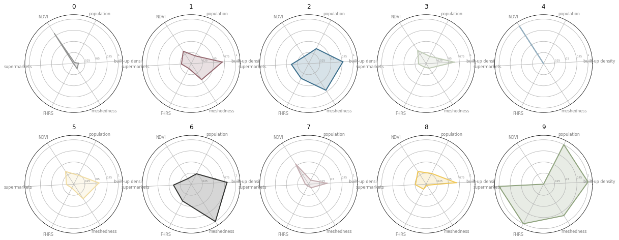
In the figure above, each score of the selected characters for each cluster is shown as a spider diagram.
fig, ax = plt.subplots(figsize=(10, 10), subplot_kw={'projection': 'polar'})

N = len(sel.columns)
angles = [(n / float(N) * 2 * np.pi)  + .05 for n in range(N)]
angles += angles[:1]

ax.set_xticks(angles[:-1])
ax.set_xticklabels(labels, color='grey', size=8)
ax.set_ylim(0, 1.1)
ax.set_yticks([.25, .5, .75, 1])
ax.set_yticklabels([.25, .5, .75, 1], color='grey', size=5)
ax.set_rlabel_position(10)
custom_points = []


for i in range(10):
    values = sel.loc[i].values.flatten().tolist()
    values += values[:1]
    ax.plot(angles, values, linewidth=2, linestyle='solid', color=cmap.colors[i])
    ax.fill(angles, values, 'b', alpha=0.05, color=cmap.colors[i])

    custom_points.append(Line2D([0], [0], marker="o", linestyle="none", markersize=5, color=cmap.colors[i]))

fig.set_facecolor('white')
leg_points = ax.legend(custom_points, range(10), loc='lower center', frameon=False, ncol=5, bbox_to_anchor=(0.5, -0.1))
ax.add_artist(leg_points)
<matplotlib.legend.Legend at 0x7fd3cfe6cd60>
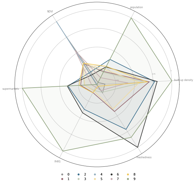
We can also overlap all clusters in the same diagram for a direct comparison.
fig, ax = plt.subplots(figsize=(10, 10), subplot_kw={'projection': 'polar'})

N = len(sel.columns)
angles = [(n / float(N) * 2 * np.pi)  + .05 for n in range(N)]
angles += angles[:1]

ax.set_xticks(angles[:-1])
ax.set_xticklabels(labels, color='grey', size=8)
ax.set_ylim(0, 1.1)
ax.set_yticks([.25, .5, .75, 1])
ax.set_yticklabels([.25, .5, .75, 1], color='grey', size=5)
ax.set_rlabel_position(10)
custom_points = []

opts = [1, 2, 6, 8, 9]

for i in opts:
    values = sel.loc[i].values.flatten().tolist()
    values += values[:1]
    ax.plot(angles, values, linewidth=2, linestyle='solid', color=cmap.colors[i])
    ax.fill(angles, values, 'b', alpha=0.05, color=cmap.colors[i])

    custom_points.append(Line2D([0], [0], marker="o", linestyle="none", markersize=5, color=cmap.colors[i]))

fig.set_facecolor('white')
leg_points = ax.legend(custom_points, opts, loc='lower center', frameon=False, ncol=5, bbox_to_anchor=(0.5, -0.1))
ax.add_artist(leg_points)
<matplotlib.legend.Legend at 0x7fd3cfce3130>
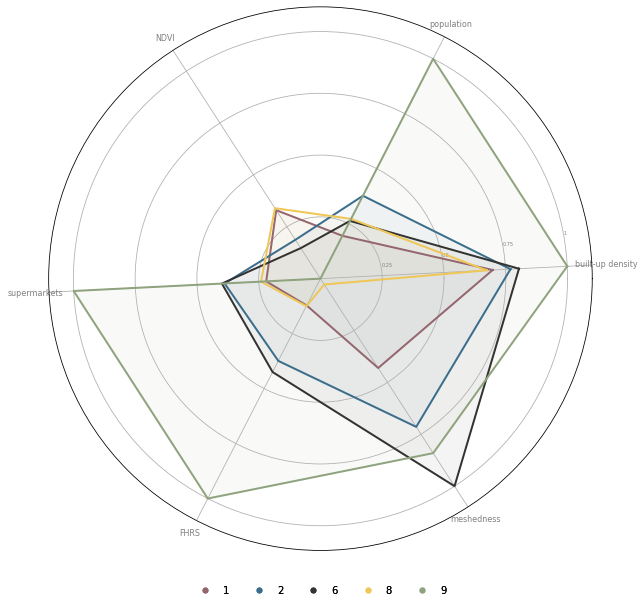
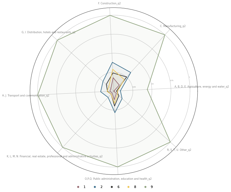
Or we can plot only the subset of clusters (urban classes here) if we want to see the differences between those.
Cluster 2 and 6 are quite similar, let’s check which characters are the most different:
(group.loc[2] - group.loc[6]).abs().sort_values()[-40:]
F. Construction_q3                      0.649119
ssbCCo_q1                               0.650907
linWID_q2                               0.656576
sdbPer_q3                               0.682242
F. Construction_q2                      0.723104
sdsSWD_q3                               0.728287
population_q3                           0.739577
population_q2                           0.749769
H, J. Transport and communication_q1    0.752492
ssbElo_q3                               0.771562
xcnSCl_q3                               0.777102
ssbCCM_q3                               0.777249
sdbAre_q2                               0.784049
ssbElo_q2                               0.796450
sdbAre_q1                               0.800752
lcdMes_q1                               0.801982
lcdMes_q3                               0.818693
lcdMes_q2                               0.838077
night_lights_q1                         0.868450
sdbPer_q1                               0.889522
night_lights_q2                         0.892386
night_lights_q3                         0.893259
ssbCCo_q3                               0.909325
sdbPer_q2                               0.917490
ssbCCo_q2                               0.921078
ssbCCM_q1                               0.950964
ssbCCM_q2                               0.991878
ltcWRE_q1                               1.198636
mtdDeg_q3                               1.199064
linP4W_q3                               1.210924
linP4W_q2                               1.240299
lteWNB_q1                               1.243230
lteWNB_q3                               1.250676
linP4W_q1                               1.292982
ltcWRE_q2                               1.372524
lteWNB_q2                               1.394225
ltcWRE_q3                               1.459551
lcnClo_q1                               1.980144
lcnClo_q2                               2.047555
lcnClo_q3                               2.127266
dtype: float64
The significant difference is in the street network patterns of both clusters. Cluster 6 is more connected, having a stronger grid-like pattern as shown in local closeness, proportion og 4-way intersections or meshedness. At the same time, it is less dense than cluster 2.
group["population_q2"]
0   -0.804873
1    0.276628
2    1.470679
3    0.198304
4   -1.000495
5    0.471169
6    0.720910
7   -0.330870
8    0.781538
9    5.556644
Name: population_q2, dtype: float64
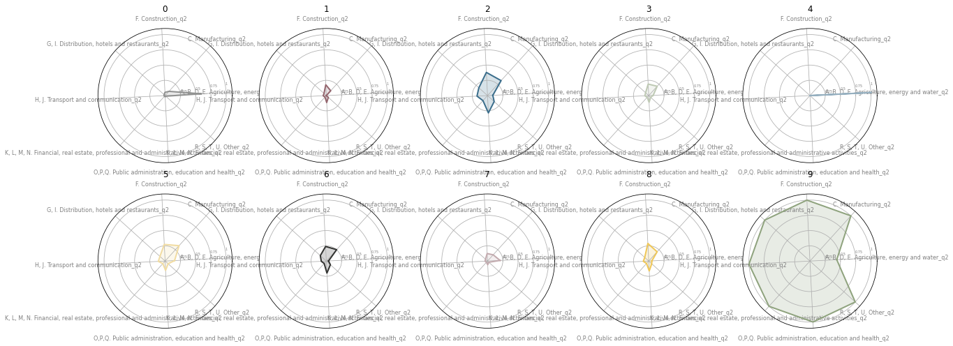
We can also check workplace population by a type of industry.
selection = ['A, B, D, E. Agriculture, energy and water_q2',
            'C. Manufacturing_q2',
            'F. Construction_q2',
            'G, I. Distribution, hotels and restaurants_q2',
            'H, J. Transport and communication_q2',
            'K, L, M, N. Financial, real estate, professional and administrative activities_q2',
            'O,P,Q. Public administration, education and health_q2',
            'R, S, T, U. Other_q2',
            ]
labels = selection

sel = group[selection]
sel = (sel-sel.min())/(sel.max()-sel.min())

fig, axs = plt.subplots(2, 5, figsize=(20, 8), subplot_kw={'projection': 'polar'})

N = len(sel.columns)
angles = [(n / float(N) * 2 * np.pi)  + .05 for n in range(N)]
angles += angles[:1]

for i, ax in enumerate(axs.flatten()):
    ax.set_xticks(angles[:-1])
    ax.set_xticklabels(labels, color='grey', size=8)
    ax.set_ylim(0, 1.1)
    ax.set_yticks([.25, .5, .75, 1])
    ax.set_yticklabels([.25, .5, .75, 1], color='grey', size=5)
    ax.set_rlabel_position(10)
    ax.set_title(i)

    values = sel.loc[i].values.flatten().tolist()
    values += values[:1]
    ax.plot(angles, values, linewidth=2, linestyle='solid', color=cmap.colors[i])
    ax.fill(angles, values, 'b', alpha=0.2, color=cmap.colors[i])

fig.set_facecolor('white')
fig, ax = plt.subplots(figsize=(10, 10), subplot_kw={'projection': 'polar'})

N = len(sel.columns)
angles = [(n / float(N) * 2 * np.pi)  + .05 for n in range(N)]
angles += angles[:1]

ax.set_xticks(angles[:-1])
ax.set_xticklabels(labels, color='grey', size=8)
ax.set_ylim(0, 1.1)
ax.set_yticks([.25, .5, .75, 1])
ax.set_yticklabels([.25, .5, .75, 1], color='grey', size=5)
ax.set_rlabel_position(10)
custom_points = []


for i in range(10):
    values = sel.loc[i].values.flatten().tolist()
    values += values[:1]
    ax.plot(angles, values, linewidth=2, linestyle='solid', color=cmap.colors[i])
    ax.fill(angles, values, 'b', alpha=0.05, color=cmap.colors[i])

    custom_points.append(Line2D([0], [0], marker="o", linestyle="none", markersize=5, color=cmap.colors[i]))

fig.set_facecolor('white')
leg_points = ax.legend(custom_points, range(10), loc='lower center', frameon=False, ncol=5, bbox_to_anchor=(0.5, -0.1))
ax.add_artist(leg_points)
<matplotlib.legend.Legend at 0x7fd3cf7458e0>
As expected, the majority of jobs is in cluster 9 (city centres), with the excepction of agriculture dominant in clusters 4 and 0.
The same data can be also plotted in an ovelapping manner for easier comparison.
fig, ax = plt.subplots(figsize=(10, 10), subplot_kw={'projection': 'polar'})

N = len(sel.columns)
angles = [(n / float(N) * 2 * np.pi)  + .05 for n in range(N)]
angles += angles[:1]

ax.set_xticks(angles[:-1])
ax.set_xticklabels(labels, color='grey', size=8)
ax.set_ylim(0, 1.1)
ax.set_yticks([.25, .5, .75, 1])
ax.set_yticklabels([.25, .5, .75, 1], color='grey', size=5)
ax.set_rlabel_position(10)
custom_points = []

opts = [1, 2, 6, 8, 9]

for i in opts:
    values = sel.loc[i].values.flatten().tolist()
    values += values[:1]
    ax.plot(angles, values, linewidth=2, linestyle='solid', color=cmap.colors[i])
    ax.fill(angles, values, 'b', alpha=0.05, color=cmap.colors[i])

    custom_points.append(Line2D([0], [0], marker="o", linestyle="none", markersize=5, color=cmap.colors[i]))

fig.set_facecolor('white')
leg_points = ax.legend(custom_points, opts, loc='lower center', frameon=False, ncol=5, bbox_to_anchor=(0.5, -0.1))
ax.add_artist(leg_points)
<matplotlib.legend.Legend at 0x7fd3cf989bb0>
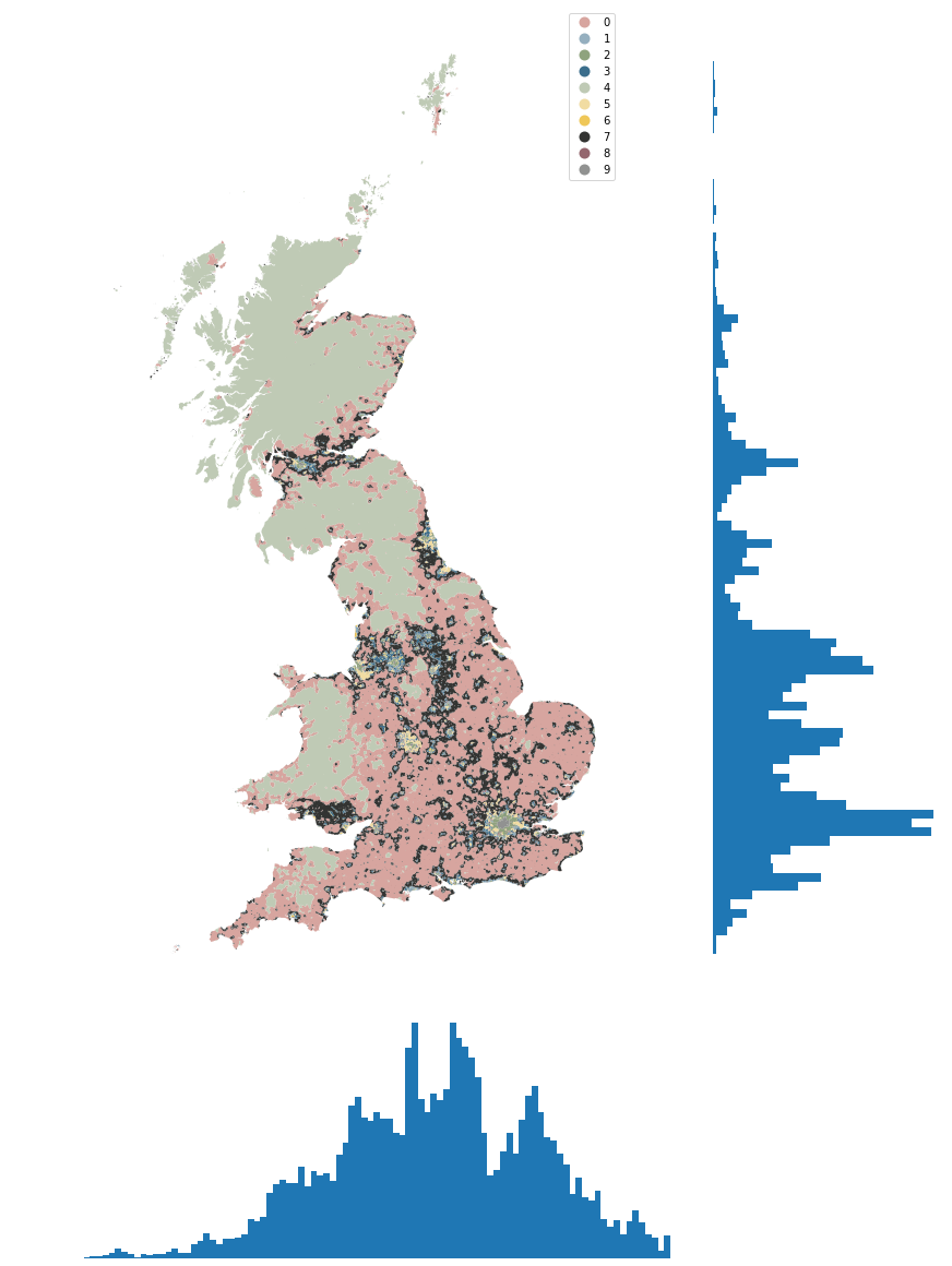
Geographical distribution
We can also check the geographical distribution of clusters.
spsig = gpd.read_parquet(f"../../urbangrammar_samba/spatial_signatures/signatures/signatures_KMeans10_GB_simplified.pq")
cmap = ugg.get_colormap(10, randomize=True)
token = ""

ax = spsig.plot("kmeans10gb", ax=axs['A'], zorder=1, linewidth=0, edgecolor='w', alpha=1, legend=True, cmap=cmap, categorical=True)
# ctx.add_basemap(ax, crs=27700, source=ugg.get_tiles('roads', token), zorder=2, alpha=.3)
# ctx.add_basemap(ax, crs=27700, source=ugg.get_tiles('labels', token), zorder=3, alpha=1)
# ctx.add_basemap(ax, crs=27700, source=ugg.get_tiles('background', token), zorder=-1, alpha=1)
ax.set_axis_off()

# plt.savefig(f"../../urbangrammar_samba/spatial_signatures/signatures/signatures_KMeans10_GB.png")
centroid = spsig.centroid
x = centroid.x
y = centroid.y
f = plt.figure(
    constrained_layout=True, figsize=(12, 16)
)
axs = f.subplot_mosaic(
    """
    AAAB
    AAAB
    AAAB
    AAAB
    CCCD
    """,
)

spsig.plot("kmeans10gb", ax=axs['A'], zorder=1, linewidth=0, edgecolor='w', alpha=1, legend=True, cmap=cmap, categorical=True)
x.plot.hist(bins=100, ax=axs["C"])
y.plot.hist(bins=100, orientation="horizontal", ax=axs["B"])
for ax in axs.values():
    ax.set_axis_off()
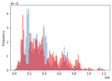
ax = y.plot.hist(bins=100, density=True, alpha=.4)
y[spsig.kmeans10gb == 4].plot.hist(bins=100, ax=ax, color='r', alpha=.5, density=True)
<AxesSubplot:ylabel='Frequency'>
spsig.kmeans10gb.value_counts()
3    17357
1    10919
0    10882
5    10675
7    10636
8     9418
2     7214
4     6214
6     2561
9     1655
Name: kmeans10gb, dtype: int64
# population by class
# calinski-harabazs per variable
# random forest and feature importance
Summary
Countryside
Clusters 0, 4, and 7 can be classified as countryside.
Cluster 0
Cluster 0 is located predominantly in England and is can be characterised as agriculture-dominated countryside. It contains both pastures and fields.
Cluster 4
Cluster 4 is the most natural of all, covering national parks and large areas of inhabited land like Scottish Highlands, Lake District or the majority of Wales.
Cluster 7
Cluster 7 can be characterised as a green belt around cities. It covers mostly agricultural land in the immediate adjacency of towns and cities, often including development on their edges.
Urban areas
The remaining classes can be classified as urban or semi-urban areas.
Periphery
Cluster 3
Cluster 3 is a transition between countryisde and urbanised land. It is located on the outskirts of cities and has typically a large open space area intertwined with different kinds of development from highways to smaller neighbourhoods. If we wanted to call an urban periphery, it would be cluster 3.
Suburbs
Clusters 1 and 8 can be described as suburban neighbourhoods. Both are on the edges of cities, both have relative lack of jobs and destinations.
Cluster 1
The main difference between them is in street networks. Cluster 1 tends to have more connected networks, even though both lack connectivty compared to some other clusters.
Cluster 8
Cluster 8 contains suburban neighbourhoods with the least connected networks.
Cities
Cluster 2 and 6 cover the majority of residential urban development, whilst cluster 9 represents dense city centers.
Cluster 2
In cluster 2 are residential neighbourhoods with some services and jobs. It is a relatively dense development, often terraced housing and other similar kinds. It is the most abundant urban cluster.
Cluster 6
Cluster 6 is very similar to the cluster 2. The main difference lies in street networks, where cluster 6 tends to have more connected grid-like patterns. However, it has less jobs than cluster 2.
Cluster 9
Cluster 9 is the dense development of city centres with an abundance of jobs and services.
Cluster 5
Finally, cluster 5 covers industrial areas in cities.