Comparison between Spatial Signatures and GHSL classes
import pandas
import geopandas
import rasterio
import xarray
import rioxarray
import xrspatial
import contextily
import dask_geopandas
import seaborn as sns
import numpy as np
import matplotlib.pyplot as plt
from geopy.geocoders import Nominatim
from shapely.geometry import box
from rasterstats import zonal_stats
from dask.array import unique as daunique
Dask setup (used in a few instances below):
from dask.distributed import Client, LocalCluster
client = Client(LocalCluster())
client
2022-07-25 08:42:48,745 - distributed.diskutils - INFO - Found stale lock file and directory '/home/jovyan/work/code/spatial_signatures/clusters/dask-worker-space/worker-_o0_mw8g', purging
2022-07-25 08:42:48,746 - distributed.diskutils - INFO - Found stale lock file and directory '/home/jovyan/work/code/spatial_signatures/clusters/dask-worker-space/worker-1o9g1gis', purging
Client
Client-c371d02d-0bf5-11ed-ad38-0242ac110002
| Connection method: Cluster object | Cluster type: distributed.LocalCluster |
| Dashboard: http://127.0.0.1:8787/status |
Cluster Info
LocalCluster
64b73a8f
| Dashboard: http://127.0.0.1:8787/status | Workers: 4 |
| Total threads: 16 | Total memory: 62.49 GiB |
| Status: running | Using processes: True |
Scheduler Info
Scheduler
Scheduler-492e68dc-dded-44c1-a7d8-509fcc1de383
| Comm: tcp://127.0.0.1:35353 | Workers: 4 |
| Dashboard: http://127.0.0.1:8787/status | Total threads: 16 |
| Started: Just now | Total memory: 62.49 GiB |
Workers
Worker: 0
| Comm: tcp://127.0.0.1:46763 | Total threads: 4 |
| Dashboard: http://127.0.0.1:33395/status | Memory: 15.62 GiB |
| Nanny: tcp://127.0.0.1:37181 | |
| Local directory: /home/jovyan/work/code/spatial_signatures/clusters/dask-worker-space/worker-h7y1drgb | |
Worker: 1
| Comm: tcp://127.0.0.1:39241 | Total threads: 4 |
| Dashboard: http://127.0.0.1:37139/status | Memory: 15.62 GiB |
| Nanny: tcp://127.0.0.1:40519 | |
| Local directory: /home/jovyan/work/code/spatial_signatures/clusters/dask-worker-space/worker-6j_mpem9 | |
Worker: 2
| Comm: tcp://127.0.0.1:46817 | Total threads: 4 |
| Dashboard: http://127.0.0.1:44471/status | Memory: 15.62 GiB |
| Nanny: tcp://127.0.0.1:45189 | |
| Local directory: /home/jovyan/work/code/spatial_signatures/clusters/dask-worker-space/worker-qevjjemv | |
Worker: 3
| Comm: tcp://127.0.0.1:37637 | Total threads: 4 |
| Dashboard: http://127.0.0.1:42319/status | Memory: 15.62 GiB |
| Nanny: tcp://127.0.0.1:39143 | |
| Local directory: /home/jovyan/work/code/spatial_signatures/clusters/dask-worker-space/worker-gjjcsw3g | |
client.restart()
Global GHSL
Read data
Global file downloaded originally from here.
ghsl_path = (
    '/home/jovyan/data/'
    'GHS_BUILT_C_MSZ_E2018_GLOBE_R2022A_54009_10_V1_0/'
    'GHS_BUILT_C_MSZ_E2018_GLOBE_R2022A_54009_10_V1_0.tif'
)
ghsl = rasterio.open(ghsl_path)
ghsl = rioxarray.open_rasterio(
    ghsl_path, chunks=11000, cache=False
)
ghsl
<xarray.DataArray (band: 1, y: 1800000, x: 3608200)>
dask.array<open_rasterio-b4b095e68e7d08b8eaf98573919622fd<this-array>, shape=(1, 1800000, 3608200), dtype=uint8, chunksize=(1, 11000, 11000), chunktype=numpy.ndarray>
Coordinates:
  * band         (band) int64 1
  * x            (x) float64 -1.804e+07 -1.804e+07 ... 1.804e+07 1.804e+07
  * y            (y) float64 9e+06 9e+06 9e+06 9e+06 ... -9e+06 -9e+06 -9e+06
    spatial_ref  int64 0
Attributes:
    _FillValue:    255.0
    scale_factor:  1.0
add_offset: 0.0Parse colors
Read and parse the color file:
def parse_clr(p):
    with open(p) as fo:
        lines = fo.readlines()
    colors = pandas.DataFrame(
        map(parse_line, lines),
        columns=['code', 'color', 'name']
    )
    return colors
def parse_line(l):
    l = l.replace('\n', '').split(' ')
    code = l[0]
    rgba = tuple(map(int, l[1:5]))
    name = ' '.join(l[5:])
    return code, rgba, name
colors = parse_clr(
    '/home/jovyan/data/GHS_BUILT_C_MSZ_E2018_GLOBE_R2022A_54009_10_V1_0/'
    'GHS_BUILT_C_MSZ_E2018_GLOBE_R2022A_54009_10_V1_0.clr'
)
Explore values
For the GB extent:
[x] What are the unique values appearing in the dataset (i.e., make sure I’m not missing anyone I don’t have now)
[x] Proportions of pixels by value (what classes are more common?)
[ ] Zoom into a few cities (e.g., London, Liverpool, Glasgow)
GB extent (hardcoded as file not read yet)
gb_bb = gb_minx, gb_miny, gb_maxx, gb_maxy = (
    -583715.9369692 , 5859449.59340008,  129491.84447583, 6958662.59197899
)
GB subset
ghsl_gb = ghsl.sel(
    x = slice(gb_minx, gb_maxx), y = slice(gb_maxy, gb_miny), band = 1
)
Unique values
We can run the set of unique values present in the GB extent.
%%time
ghsl_class_values = daunique(ghsl_gb.data).compute()
ghsl_class_values
CPU times: user 2.22 s, sys: 238 ms, total: 2.45 s
Wall time: 20.5 s
array([  0,   1,   2,   3,   4,   5,  11,  12,  13,  14,  15,  21,  22,
        23,  24,  25, 255], dtype=uint8)
This shows that, compared to the color files (parsed above), there are only two additional values present in the dataset: 0, which we later name as “Other” (although it is unclear what it represents); and 255, which is the value for missing data/NaN.
Proportions
Now we are interested in knowing how prevalent each class/value is acros GB.
%%time
proportions = xrspatial.zonal.stats(
    zones=ghsl_gb, values=ghsl_gb, stats_funcs=['count']
).compute()
proportions
/opt/conda/lib/python3.9/site-packages/dask/dataframe/multi.py:1254: UserWarning: Concatenating dataframes with unknown divisions.
We're assuming that the indices of each dataframes are
 aligned. This assumption is not generally safe.
  warnings.warn(
CPU times: user 1min 27s, sys: 5.73 s, total: 1min 33s
Wall time: 4min 36s
| zone | count | |
|---|---|---|
| 0 | 0 | 5.602494e+09 |
| 1 | 1 | 7.034046e+06 |
| 2 | 2 | 2.815456e+07 |
| 3 | 3 | 6.134572e+07 |
| 4 | 4 | 5.850830e+05 |
| 5 | 5 | 5.812731e+06 |
| 6 | 11 | 3.165273e+07 |
| 7 | 12 | 1.810498e+07 |
| 8 | 13 | 3.299108e+07 |
| 9 | 14 | 9.017500e+05 |
| 10 | 15 | 2.023200e+04 |
| 11 | 21 | 1.582956e+06 |
| 12 | 22 | 1.108482e+06 |
| 13 | 23 | 5.876578e+06 |
| 14 | 24 | 6.344250e+05 |
| 15 | 25 | 3.404800e+04 |
| 16 | 255 | 2.041342e+09 |
Now build a crosswalk for the names:
cw = colors.set_index('code').rename(int)['name']
cw.loc[0] = 'Other'
cw.loc[255] = 'N/A'
And display in a bar plot (removing Other and N/A):
count = proportions.assign(
    zone_name=proportions['zone'].map(cw)
).set_index(
    'zone_name'
)
(
    count[['count']] * 100 / count['count'].sum()
).sort_values(
    'count'
).drop(
    ['N/A', 'Other']
)['count'].plot.bar(
    figsize=(12, 6), title='Class proportions in GB'
)
plt.xticks(
    rotation=45,
    horizontalalignment='right',
    fontweight='light',
    fontsize='medium',
);
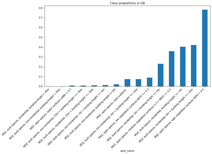
Note this tops at less than 1% of land. The other two categories take the rest:
(
    count[['count']] * 100 / count['count'].sum()
).loc[['Other', 'N/A']]
| count | |
|---|---|
| zone_name | |
| Other | 71.463343 |
| N/A | 26.038602 |
Visualisations
Let’s manually get extents for a few cities:
city_names = ['London', 'Liverpool', 'Glasgow']
cities = geopandas.GeoSeries(
    pandas.concat([name2poly(city) for city in city_names]).values, index=city_names,
).to_crs(ghsl.rio.crs)
cities
London       POLYGON ((24970.789 6007550.107, 24830.971 604...
Liverpool    POLYGON ((-204665.595 6215723.946, -204168.578...
Glasgow      POLYGON ((-286155.194 6456752.478, -284662.788...
dtype: geometry
A few tools…
def colorify_ghsl(da, cw):
'''
Generate plot of GHSL map using official color coding
'''
# Generate output array with same XY dimensions and a third one
out = xarray.DataArray(
np.zeros((4, *da.shape), dtype=da.dtype),
coords={'y': da.coords['y'], 'x': da.coords['x'], 'band': [1, 2, 3, 4]},
dims=['band', 'y', 'x']
)
# Loop over each color
for code, color in cw.iteritems():
# Find XY indices where code is found
# Assign color in those locations
out = xarray.where(
da == int(code),
xarray.DataArray(np.array(color), [[1, 2, 3, 4]], ['band']),
out
)
# Return output array
return out
cw = colors.set_index('code')['color']
def extract_city(minx, miny, maxx, maxy):
out = ghsl_gb.sel(
x=slice(minx, maxx), y=slice(maxy, miny)
).compute()
return out
geolocator = Nominatim(user_agent="dab_research").geocode
def name2poly(name):
loc = geolocator(name)
miny, maxy, minx, maxx = tuple(map(float, loc.raw['boundingbox']))
poly = geopandas.GeoSeries([box(minx, miny, maxx, maxy)], crs='EPSG:4326')
return poly
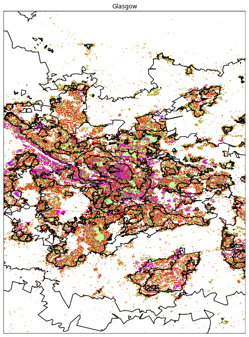
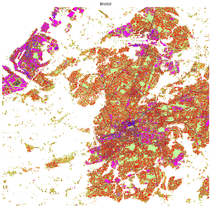
def map_city(name, cw=cw, linewidth=0.5, figsize=(12, 12)):
da = extract_city(*name2poly(name).to_crs(ghsl_gb.rio.crs).total_bounds)
xmin, ymin, xmax, ymax = da.rio.bounds()
f, ax = plt.subplots(1, figsize=figsize)
colorify_ghsl(da, cw).plot.imshow(ax=ax)
ss.clip(box(xmin, ymin, xmax, ymax)).plot(
facecolor='none', linewidth=linewidth, ax=ax
)
ax.set_title(name)
ax.set_axis_off()
return plt.show()
And we can plot all cities:
%matplotlib ipympl
Warning: Cannot change to a different GUI toolkit: ipympl. Using notebook instead.
map_city('Liverpool', linewidth=0.5)
map_city('London', figsize=(6, 6), linewidth=0)
map_city('Glasgow')
map_city('Bristol', linewidth=0)
Spatial Signatures
Read data
We use the officially released file with all detail (and a larger footprint) is available from the Figshare repository here.
ss = geopandas.read_file(
    '/home/jovyan/data/spatial_signatures/'
    'spatial_signatures_GB.gpkg'
).to_crs(ghsl.rio.crs)
Build list of types to turn them into ints:
types = {i: j[1]['type'] for i, j in enumerate(
    ss[['code', 'type']].drop_duplicates().iterrows()
)}
types_r = {types[i]: i for i in types}
types
{0: 'Countryside agriculture',
 1: 'Accessible suburbia',
 2: 'Open sprawl',
 3: 'Wild countryside',
 4: 'Warehouse/Park land',
 5: 'Gridded residential quarters',
 6: 'Urban buffer',
 7: 'Disconnected suburbia',
 8: 'Dense residential neighbourhoods',
 9: 'Connected residential neighbourhoods',
 10: 'Dense urban neighbourhoods',
 11: 'Local urbanity',
 12: 'Concentrated urbanity',
 13: 'Regional urbanity',
 14: 'outlier',
 15: 'Metropolitan urbanity',
 16: 'Hyper concentrated urbanity'}
Add column with class int:
ss['code_no'] = ss['type'].map(types_r)
Explore areas
Calculate the area
ss['area'] = ss.area
The distribution is heavily skewed, with five polygons above 1e10. Kicking out ten polygons gets the largest area within 0.5 * 1e10:
ax0 = ss['area'].plot.hist(bins=300, figsize=(12, 3))
sns.rugplot(ss['area'], color='r', alpha=1, ax=ax0);
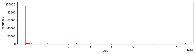
Subset to remove the largest ten signatures:
sub = ss.sort_values(
    'area', ascending=False
).iloc[10:, :]
They all belong in the least urban classes:
ss.sort_values(
    'area', ascending=False
).head(10)['type'].unique()
array(['Countryside agriculture', 'Wild countryside', 'Urban buffer'],
      dtype=object)
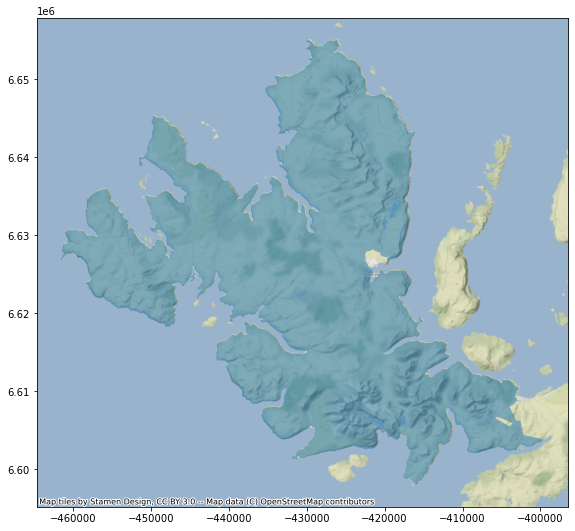
We can now explore the largest remaining polygons:
ax = sub.head(1).plot(alpha=0.5, figsize=(12, 9))
contextily.add_basemap(ax, crs=sub.crs);
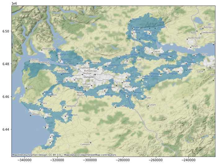
ax = sub.iloc[[1], :].plot(alpha=0.5, figsize=(12, 9))
contextily.add_basemap(ax, crs=sub.crs);
CONCLUSION - A pragmatic approach is to remove the ten largest signature polygons and run on Dask zonal stats, then process individually, with all memory dedicated to each job, each of the remaining ones, and finally merge the set.
Overlap
The strategy to obtain the overlap on all signature polygons is the following:
[x] Run on Dask overlap for all but the largest ten areas in small partitions
[x] For larger polygons:
Split polygon into smaller ones by overlaying a grid of a given size (
griddify)Assign IDs that allow to reconstruct zonal stats
Run on Dask
Collect and aggregate at the original signature level
[x] Merge all area overlap into a single table
[x] Reindex to align with
ss[x] Write down to file
Smaller areas
Move smaller signatures to Dask:
ss_ddf = dask_geopandas.from_geopandas(
    ss.sort_values('area').iloc[:-10, :],
    chunksize=1000
)
Preliminaries. We get the names as category_map so the output is expressed with class names from GHSL. It is important to note that there is an additional category that does not appear in the color file, 0, which we name as “Other”.
category_map = colors.assign(code=colors['code'].astype(int)).set_index('code')['name'].to_dict()
category_map[0] = 'Other'

def do_zonal_stats(df):
    out = zonal_stats(
        df,
        ghsl_path,
        categorical=True,
        category_map=category_map,
        all_touched=True
    )
    out = pandas.DataFrame(out).reindex(
        columns=category_map.values()
    )
    out['id'] = df['id'].values
    return out

meta = {c: 'str' for c in category_map.values()}
meta['id'] = 'str'
Build computation graph for all but the largest areas:
tmp = ss_ddf.map_partitions(
    do_zonal_stats,
    meta=meta
)
Execute on Dask cluster:
%%time
out = tmp.compute()
out.to_parquet('/home/jovyan/data/spatial_signatures/ghsl_proportions.pq')
ERROR 1: PROJ: proj_create_from_database: Open of /opt/conda/share/proj failed
ERROR 1: PROJ: proj_create_from_database: Open of /opt/conda/share/proj failed
ERROR 1: PROJ: proj_create_from_database: Open of /opt/conda/share/proj failed
ERROR 1: PROJ: proj_create_from_database: Open of /opt/conda/share/proj failed
CPU times: user 9min 17s, sys: 52.8 s, total: 10min 10s
Wall time: 1h 9s
Largest areas
Method to split up a polygon into chunks by overlaying a grid with either cells cells, or cells of side side:
def griddify(poly, side=None, cells=None, pid=None, crs=None):
    minx, miny, maxx, maxy = poly.bounds
    if side is not None:
        xs = np.arange(minx, maxx+side, side)
        ys = np.arange(miny, maxy+side, side)
    elif cells is not None:
        xs = np.linspace(minx, maxx, cells)
        ys = np.linspace(miny, maxy, cells)
    else:
        raise Exception(
            "Please make either `side` or `cells` not None"
        )
    geoms = []
    for i in range(len(xs)-1):
        for j in range(len(ys)-1):
            geoms.append(box(xs[i], ys[j], xs[i+1], ys[j+1]))
    grid = geopandas.GeoDataFrame(
        {'geometry': geoms, 'subdivision': np.arange(len(geoms))},
        crs=crs
    )
    if pid is not None:
        grid['sid'] = pid
    grid = geopandas.overlay(
        grid, geopandas.GeoDataFrame({'geometry':[poly]}, crs=crs)
    )
    return grid
Pick the largest ten that have not been already processed:
largest = ss.sort_values('area').tail(10)
Subdivide them into smaller chunks that can be easily processed in Dask:
%%time
subdivided = pandas.concat(
    largest.apply(
        lambda r: griddify(r['geometry'], side=10000, pid=r['id'], crs=ss.crs),
        axis=1
    ).tolist()
)
CPU times: user 7min 31s, sys: 439 ms, total: 7min 32s
Wall time: 7min 10s
Ship subdivided to Dask and build computation graph:
client.restart()
2022-07-25 09:52:56,773 - distributed.nanny - WARNING - Restarting worker
2022-07-25 09:52:56,775 - distributed.nanny - WARNING - Restarting worker
2022-07-25 09:52:56,983 - distributed.nanny - WARNING - Restarting worker
2022-07-25 09:52:56,984 - distributed.nanny - WARNING - Restarting worker
Client
Client-c371d02d-0bf5-11ed-ad38-0242ac110002
| Connection method: Cluster object | Cluster type: distributed.LocalCluster |
| Dashboard: http://127.0.0.1:8787/status |
Cluster Info
LocalCluster
64b73a8f
| Dashboard: http://127.0.0.1:8787/status | Workers: 4 |
| Total threads: 16 | Total memory: 62.49 GiB |
| Status: running | Using processes: True |
Scheduler Info
Scheduler
Scheduler-492e68dc-dded-44c1-a7d8-509fcc1de383
| Comm: tcp://127.0.0.1:35353 | Workers: 4 |
| Dashboard: http://127.0.0.1:8787/status | Total threads: 16 |
| Started: 1 hour ago | Total memory: 62.49 GiB |
Workers
Worker: 0
| Comm: tcp://127.0.0.1:33651 | Total threads: 4 |
| Dashboard: http://127.0.0.1:32891/status | Memory: 15.62 GiB |
| Nanny: tcp://127.0.0.1:37181 | |
| Local directory: /home/jovyan/work/code/spatial_signatures/clusters/dask-worker-space/worker-qxf30f6m | |
Worker: 1
| Comm: tcp://127.0.0.1:43355 | Total threads: 4 |
| Dashboard: http://127.0.0.1:43649/status | Memory: 15.62 GiB |
| Nanny: tcp://127.0.0.1:40519 | |
| Local directory: /home/jovyan/work/code/spatial_signatures/clusters/dask-worker-space/worker-jhqountl | |
Worker: 2
| Comm: tcp://127.0.0.1:33891 | Total threads: 4 |
| Dashboard: http://127.0.0.1:40653/status | Memory: 15.62 GiB |
| Nanny: tcp://127.0.0.1:45189 | |
| Local directory: /home/jovyan/work/code/spatial_signatures/clusters/dask-worker-space/worker-0epiev46 | |
Worker: 3
| Comm: tcp://127.0.0.1:35651 | Total threads: 4 |
| Dashboard: http://127.0.0.1:35451/status | Memory: 15.62 GiB |
| Nanny: tcp://127.0.0.1:39143 | |
| Local directory: /home/jovyan/work/code/spatial_signatures/clusters/dask-worker-space/worker-wsp2ejeu | |
subdivided['id'] = subdivided['subdivision'].astype(str) + '-' + subdivided['sid']

largest_ddf = dask_geopandas.from_geopandas(subdivided, chunksize=100)
tmp = largest_ddf.map_partitions(do_zonal_stats, meta=meta)
Run computation on Dask cluster:
%%time
subdivided_stats = tmp.compute()
ERROR 1: PROJ: proj_create_from_database: Open of /opt/conda/share/proj failed
ERROR 1: PROJ: proj_create_from_database: Open of /opt/conda/share/proj failed
ERROR 1: PROJ: proj_create_from_database: Open of /opt/conda/share/proj failed
ERROR 1: PROJ: proj_create_from_database: Open of /opt/conda/share/proj failed
/opt/conda/lib/python3.9/site-packages/geopandas/_vectorized.py:153: ShapelyDeprecationWarning: __len__ for multi-part geometries is deprecated and will be removed in Shapely 2.0. Check the length of the `geoms` property instead to get the  number of parts of a multi-part geometry.
  out[:] = [_pygeos_to_shapely(geom) for geom in data]
CPU times: user 17.9 s, sys: 1.46 s, total: 19.3 s
Wall time: 1min 44s
Aggregate at signature level by adding up values in each signature:
subdivided_stats['sid'] = subdivided_stats['id'].map(lambda i: i.split('-')[1])
largest_stats = subdivided_stats.groupby('sid').sum().reset_index()
largest_stats
| sid | MSZ, open spaces, low vegetation surfaces NDVI <= 0.3 | MSZ, open spaces, medium vegetation surfaces 0.3 < NDVI <= 0.5 | MSZ, open spaces, high vegetation surfaces NDVI > 0.5 | MSZ, open spaces, water surfaces LAND < 0.5 | MSZ, open spaces, road surfaces | MSZ, built spaces, residential, building height <= 3m | MSZ, built spaces, residential, 3m < building height <= 6m | MSZ, built spaces, residential, 6m < building height <= 15m | MSZ, built spaces, residential, 15m < building height <= 30m | MSZ, built spaces, residential, building height > 30m | MSZ, built spaces, non-residential, building height <=3m | MSZ, built spaces, non-residential, 3m < building height <= 6m | MSZ, built spaces, non-residential, 6m < building height <= 15m | MSZ, built spaces, non-residential, 15m < building height <= 30m | MSZ, built spaces, non-residential, building height > 30m | Other | |
|---|---|---|---|---|---|---|---|---|---|---|---|---|---|---|---|---|---|
| 0 | 39193_WIC | 1138.0 | 4695.0 | 29653.0 | 293.0 | 2680.0 | 39921.0 | 0.0 | 0.0 | 0.0 | 0.0 | 657.0 | 0.0 | 0.0 | 0.0 | 0.0 | 19118831.0 |
| 1 | 39251_WIC | 23390.0 | 162111.0 | 527781.0 | 7478.0 | 40714.0 | 786886.0 | 3065.0 | 1320.0 | 120.0 | 0.0 | 32795.0 | 1629.0 | 1142.0 | 1245.0 | 0.0 | 392963527.0 |
| 2 | 39497_WIC | 4663.0 | 35640.0 | 432333.0 | 1277.0 | 24170.0 | 554649.0 | 7900.0 | 1061.0 | 0.0 | 0.0 | 14591.0 | 890.0 | 1118.0 | 0.0 | 0.0 | 100484844.0 |
| 3 | 39729_WIC | 9172.0 | 100903.0 | 705946.0 | 7632.0 | 40268.0 | 857290.0 | 67438.0 | 5778.0 | 0.0 | 0.0 | 80755.0 | 7440.0 | 2076.0 | 0.0 | 0.0 | 236194274.0 |
| 4 | 459_COA | 176010.0 | 1790322.0 | 10428891.0 | 57371.0 | 582534.0 | 10768204.0 | 1778848.0 | 299119.0 | 14779.0 | 964.0 | 611600.0 | 153111.0 | 286784.0 | 32264.0 | 3387.0 | 719705569.0 |
| 5 | 479_COA | 5625.0 | 53297.0 | 165588.0 | 3346.0 | 16150.0 | 171664.0 | 68041.0 | 11930.0 | 152.0 | 73.0 | 15540.0 | 8060.0 | 8330.0 | 161.0 | 387.0 | 17453666.0 |
| 6 | 583_COA | 6937.0 | 71197.0 | 208668.0 | 2547.0 | 18409.0 | 266114.0 | 15827.0 | 4480.0 | 657.0 | 0.0 | 24492.0 | 2896.0 | 2446.0 | 800.0 | 0.0 | 26316439.0 |
| 7 | 60230_URB | 51906.0 | 302911.0 | 501268.0 | 6821.0 | 57306.0 | 383084.0 | 283760.0 | 168444.0 | 2876.0 | 0.0 | 15713.0 | 20852.0 | 48599.0 | 8086.0 | 0.0 | 16541750.0 |
| 8 | 63883_URB | 125007.0 | 797047.0 | 1543231.0 | 21005.0 | 139818.0 | 772403.0 | 959215.0 | 566485.0 | 3029.0 | 86.0 | 65965.0 | 83668.0 | 215883.0 | 5875.0 | 636.0 | 36155195.0 |
| 9 | 66140_URB | 83158.0 | 546579.0 | 1911597.0 | 11646.0 | 126916.0 | 835693.0 | 1073994.0 | 382943.0 | 3408.0 | 184.0 | 44970.0 | 52928.0 | 109235.0 | 4767.0 | 0.0 | 30507595.0 |
Merge areas and write out
smallest_stats = pandas.read_parquet(
    '/home/jovyan/data/spatial_signatures/ghsl_proportions.pq'
).rename(columns={'id': 'sid'})
all_stats = pandas.concat([smallest_stats, largest_stats])
ss.join(
    all_stats.set_index('sid'), on='id'
).to_parquet(
    '/home/jovyan/data/spatial_signatures/ghsl_proportion_stats.pq'
)
/tmp/ipykernel_1027384/1151739440.py:1: UserWarning: this is an initial implementation of Parquet/Feather file support and associated metadata.  This is tracking version 0.1.0 of the metadata specification at https://github.com/geopandas/geo-arrow-spec

This metadata specification does not yet make stability promises.  We do not yet recommend using this in a production setting unless you are able to rewrite your Parquet/Feather files.

To further ignore this warning, you can do:
import warnings; warnings.filterwarnings('ignore', message='.*initial implementation of Parquet.*')
  ss.join(
Comparison
sso = geopandas.read_parquet(
    '/home/jovyan/data/spatial_signatures/ghsl_proportion_stats.pq'
)
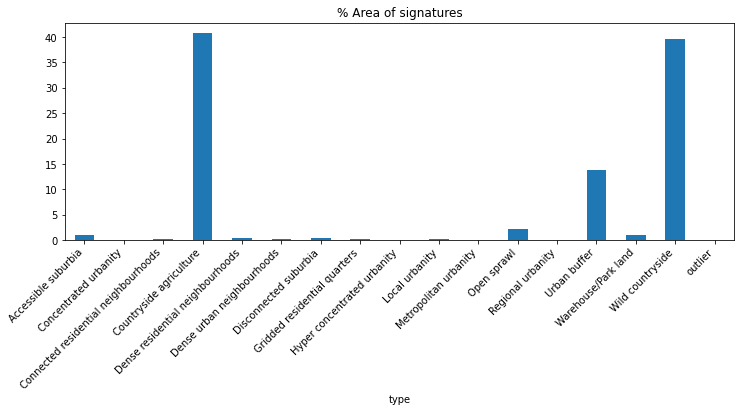
Proportions of signatures by area covered
(
    sso.groupby('type').sum()['area'] * 100 /
    sso.groupby('type').sum()['area'].sum()
).plot.bar(figsize=(12, 4), title="% Area of signatures")
plt.xticks(
    rotation=45,
    horizontalalignment='right',
    fontweight='light',
    fontsize='medium',
);
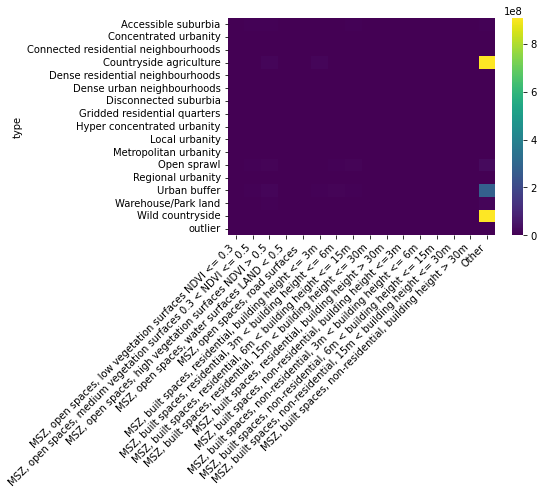
And we can turn to overlap across classes. We start with an overall comparison:
sns.heatmap(
    sso.groupby('type').sum().loc[
        :, 'MSZ, open spaces, low vegetation surfaces NDVI <= 0.3':
    ],
    cmap='viridis'
)
plt.xticks(
    rotation=45,
    horizontalalignment='right',
    fontweight='light',
    fontsize='medium',
);
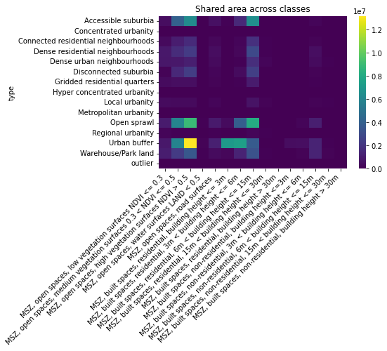
And, perhaps more interestingly, how the rest of classes then relate to each other:
ax = sns.heatmap(
    sso.groupby('type').sum().loc[
        :, 'MSZ, open spaces, low vegetation surfaces NDVI <= 0.3':
    ].drop(
        index=['Wild countryside', 'Countryside agriculture'], columns=['Other']
    ),
    cmap='viridis',
)
ax.set_title('Shared area across classes')
plt.xticks(
    rotation=45,
    horizontalalignment='right',
    fontweight='light',
    fontsize='medium',
);
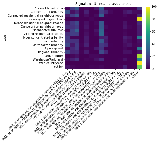
This is still hard to see clear patterns, let’s turn to proportions. We can look at what proportions of each signature class end up in GHSL classes:
tmp = sso.groupby('type').sum().loc[
    :, 'MSZ, open spaces, low vegetation surfaces NDVI <= 0.3':
]

ax = sns.heatmap(
    (tmp * 100).div(tmp.sum(axis=1), axis=0),
    cmap='viridis',
    vmin=0,
    vmax=100
)
ax.set_title('Signature % area across classes')
plt.xticks(
    rotation=45,
    horizontalalignment='right',
    fontweight='light',
    fontsize='medium',
);
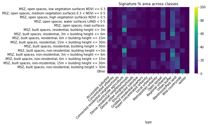
And, viceversa, how much of a GHSL class ends up in Signature classes:
tmp = sso.groupby('type').sum().loc[
    :, 'MSZ, open spaces, low vegetation surfaces NDVI <= 0.3':
].T

ax = sns.heatmap(
    (tmp * 100).div(tmp.sum(axis=1), axis=0),
    cmap='viridis',
    vmin=0,
    vmax=100
)
ax.set_title('Signature % area across classes')
plt.xticks(
    rotation=45,
    horizontalalignment='right',
    fontweight='light',
    fontsize='medium',
);
DEPRECATED
As of July 13th’22, the approaches below are deprecated because loading imagery for certain signature polygons is deemed unfeasible. The main issue is there are a few very large polygons:
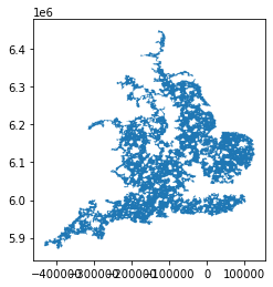
ssa = ss.area
ss[ssa == ssa.max()].plot();
Single-core approach
%%time
stats = pandas.DataFrame(
    zonal_stats(ss.head(100), ghsl_path, categorical=True),
).reindex(columns=colors['code'].astype(int))
CPU times: user 3.14 s, sys: 15.1 s, total: 18.3 s
Wall time: 18.1 s
Signature rasterisation
Following similar procedures (e.g., here), we rasterise the signatures.
%%time
rss = make_geocube(
    ss,
    measurements=['code_no'],
    like=ghsl.rio.clip_box(*ss.total_bounds)
)
rss
<xarray.Dataset>
Dimensions:      (y: 109923, x: 71322)
Coordinates:
  * y            (y) float64 6.959e+06 6.959e+06 ... 5.859e+06 5.859e+06
  * x            (x) float64 -5.837e+05 -5.837e+05 ... 1.295e+05 1.295e+05
    spatial_ref  int64 0
Data variables:
*empty*ghsl.rio.clip_box(*ss.total_bounds)
<xarray.DataArray (band: 1, y: 109923, x: 71322)>
dask.array<getitem, shape=(1, 109923, 71322), dtype=uint8, chunksize=(1, 11000, 11000), chunktype=numpy.ndarray>
Coordinates:
  * band         (band) int64 1
  * x            (x) float64 -5.837e+05 -5.837e+05 ... 1.295e+05 1.295e+05
  * y            (y) float64 6.959e+06 6.959e+06 ... 5.859e+06 5.859e+06
    spatial_ref  int64 0
Attributes:
    scale_factor:  1.0
    add_offset:    0.0
    _FillValue:    255