Generate Spatial Signatures across GB
This notebook generates spatial signatures as a clustering of form and function characters.
Number of clusters
Clustergram which will be used to determine number of clusters will likely be complex. It is better to use new interactive version (clustergram=>0.5.0 required).
# pip install git+https://github.com/martinfleis/clustergram.git
import dask.dataframe
import numpy as np

from clustergram import Clustergram
We first load all standardized data and create a single pandas DataFrame.
standardized_form = dask.dataframe.read_parquet("../../urbangrammar_samba/spatial_signatures/clustering_data/form/standardized/").set_index('hindex')
stand_fn = dask.dataframe.read_parquet("../../urbangrammar_samba/spatial_signatures/clustering_data/function/standardized/")
data = dask.dataframe.multi.concat([standardized_form, stand_fn], axis=1).replace([np.inf, -np.inf], np.nan).fillna(0)
%time data = data.compute()
CPU times: user 2min 36s, sys: 1min 24s, total: 4min
Wall time: 2min 43s
Due to a small mistake, parquet files contain 3 columns which were used temporarily during the computation. We remove them now.
data = data.drop(columns=["keep_q1", "keep_q2", "keep_q3"])
We run clustergram for all the options between 1 and 24 clusters using Mini-Batch K-Means algorithm.
cgram = Clustergram(range(1, 25), method='minibatchkmeans', batch_size=1_000_000, n_init=100, random_state=42)
cgram.fit(data)
K=1 fitted in 780.0785899162292 seconds.
K=2 fitted in 864.1424376964569 seconds.
K=3 fitted in 954.2592947483063 seconds.
K=4 fitted in 1258.9098596572876 seconds.
K=5 fitted in 1360.8928196430206 seconds.
K=6 fitted in 1446.0337007045746 seconds.
K=7 fitted in 1550.0224254131317 seconds.
K=8 fitted in 1662.5290818214417 seconds.
K=9 fitted in 1759.5144119262695 seconds.
K=10 fitted in 1860.4208154678345 seconds.
K=11 fitted in 1957.2675037384033 seconds.
K=12 fitted in 2036.3741669654846 seconds.
K=13 fitted in 2098.1098449230194 seconds.
K=14 fitted in 2188.7303895950317 seconds.
K=15 fitted in 2251.541695833206 seconds.
K=16 fitted in 2390.264476776123 seconds.
K=17 fitted in 2506.9812376499176 seconds.
K=18 fitted in 2602.7613401412964 seconds.
K=19 fitted in 2642.102708339691 seconds.
K=20 fitted in 2746.4516792297363 seconds.
K=21 fitted in 2901.3386924266815 seconds.
K=22 fitted in 3010.796851873398 seconds.
K=23 fitted in 3055.145115852356 seconds.
K=24 fitted in 3155.7938318252563 seconds.
We can save resulting labels to parquet.
labels = cgram.labels.copy()
labels.columns = labels.columns.astype("str")  # parquet require str column names
labels.to_parquet("../../urbangrammar_samba/spatial_signatures/clustering_data/clustergram_labels.pq")
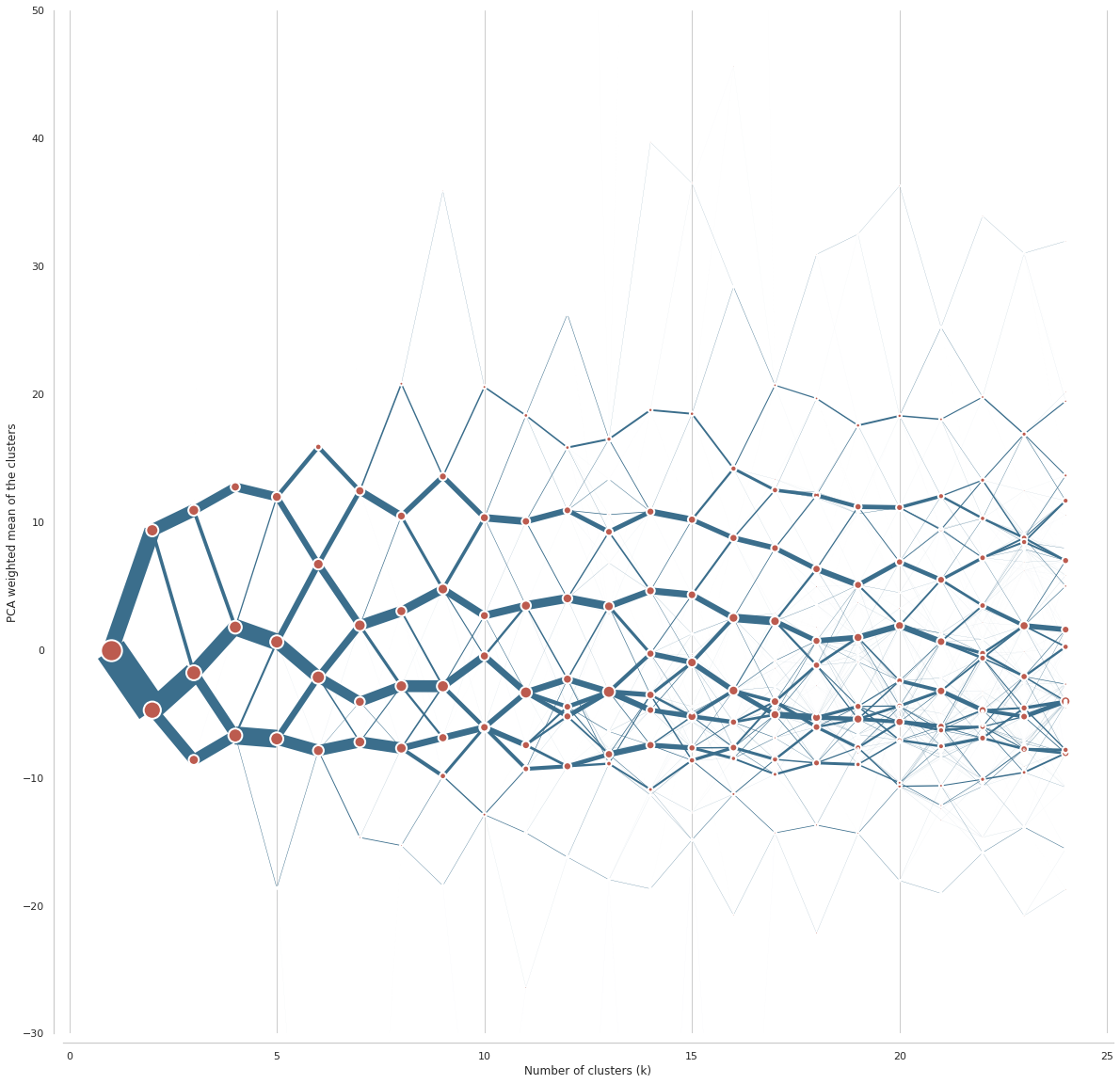
Now we can plot the clustergram.
import urbangrammar_graphics as ugg
import seaborn as sns

sns.set(style='whitegrid')
%%time

ax = cgram.plot(
    figsize=(20, 20),
    line_style=dict(color=ugg.COLORS[1]),
    cluster_style={"color": ugg.COLORS[2]},
)
ax.yaxis.grid(False)
sns.despine(offset=10)
ax.set_ylim(-30, 50)
CPU times: user 11min 28s, sys: 4min 51s, total: 16min 20s
Wall time: 3min 30s
(-30.0, 50.0)
Better option is an interactive clustergram, showing the same data in a more friendly manner. We first initialise bokeh.
from bokeh.io import output_notebook
from bokeh.plotting import show

output_notebook()
Now we can plot clustergram using bokeh. First the same as above, using PCA weighting.
fig = cgram.bokeh(
    figsize=(800, 600),
    line_style=dict(color=ugg.HEX[1]),
    cluster_style={"color": ugg.HEX[2]},
)
show(fig)
Second, we can plot clustergram using mean values. Both perspectives combined give us a better picture of clustering behaviour.
fig2 = cgram.bokeh(
    figsize=(800, 600),
    line_style=dict(color=ugg.HEX[1]),
    cluster_style={"color": ugg.HEX[2]},
    pca_weighted=False
)
show(fig2)
cgram.labels[10].value_counts()
5    3336758
4    2703587
3    2610026
1    2564843
6    2350191
0     486626
2     483285
8       3714
7        545
9          3
Name: 10, dtype: int64
Clustergram is one way of determination of number of clusters. It is always better to use more options.
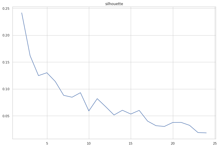
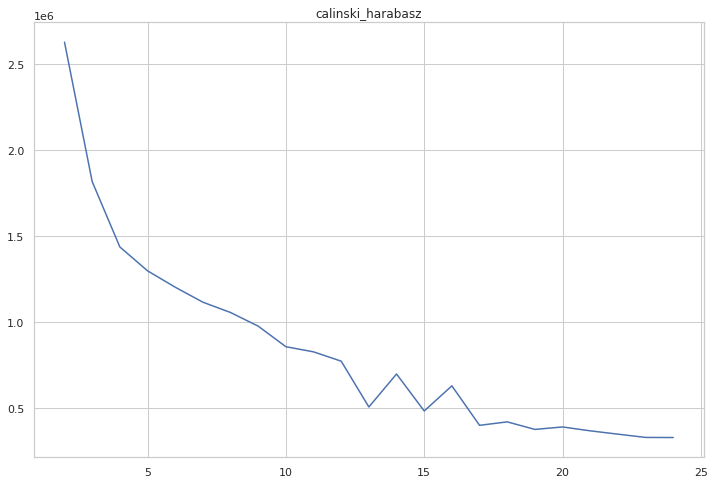
Here we automatically compute mean silhouette scores, Calinski-Harabasz scores and Davies-Bouldin scores from clustergram.
cgram.silhouette_score(sample_size=100_000)
cgram.silhouette.plot(figsize=(12, 8), title="silhouette")
<AxesSubplot:title={'center':'silhouette'}>
cgram.calinski_harabasz_score()
cgram.calinski_harabasz.plot(figsize=(12, 8), title="calinski_harabasz")
<AxesSubplot:title={'center':'calinski_harabasz'}>
cgram.davies_bouldin_score()
cgram.davies_bouldin.plot(figsize=(12, 8), title="davies_bouldin")
<AxesSubplot:title={'center':'davies_bouldin'}>
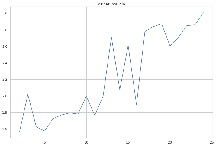
All diagrams combined point to 10 clusters as an optimal solution.
We can save clustrgram object for later reuse (note that is is large as is contains the data).
import pickle

with open('../../urbangrammar_samba/spatial_signatures/clustering_data/clustergram.pickle','wb') as f:
    pickle.dump(cgram, f)
We can also use labels from the clustergram to create provisional maps of signatures.
import geopandas as gpd
import matplotlib.pyplot as plt
import contextily as ctx
import urbangrammar_graphics as ugg
import dask_geopandas
from utils.dask_geopandas import dask_dissolve
We load data for two chunks, assing labels and dissolve tessellation cells to signatures (using dask).
geom51 = gpd.read_parquet("../../urbangrammar_samba/spatial_signatures/tessellation/tess_51.pq", columns=["tessellation", "hindex"])
geom68 = gpd.read_parquet("../../urbangrammar_samba/spatial_signatures/tessellation/tess_68.pq", columns=["tessellation", "hindex"])
labels.index = data.index
geom51 = geom51.set_index("hindex")
geom51["cluster"] = labels["11"].loc[labels.index.str.startswith("c051")]
geom68 = geom68.set_index("hindex")
geom68["cluster"] = labels["11"].loc[labels.index.str.startswith("c068")]
cmap = ugg.get_colormap(16, randomize=True)

for i, geom in enumerate([geom51, geom68]):
    ddf = dask_geopandas.from_geopandas(geom.sort_values('cluster'), npartitions=64)
    spsig = dask_dissolve(ddf, by='cluster').compute().reset_index(drop=True).explode()

    token = ""

    ax = spsig.plot("cluster", figsize=(20, 20), zorder=1, linewidth=.3, edgecolor='w', alpha=1, legend=True, cmap=cmap, categorical=True)
    ctx.add_basemap(ax, crs=27700, source=ugg.get_tiles('roads', token), zorder=2, alpha=.3)
    ctx.add_basemap(ax, crs=27700, source=ugg.get_tiles('labels', token), zorder=3, alpha=1)
    ctx.add_basemap(ax, crs=27700, source=ugg.get_tiles('background', token), zorder=-1, alpha=1)
    ax.set_axis_off()

    plt.savefig(f"../../urbangrammar_samba/spatial_signatures/clustering_data/validation/maps/fixed_option11_{i}.png")
    plt.close()
We do the same for one more chunk representing central London.
geom15 = gpd.read_parquet("../../urbangrammar_samba/spatial_signatures/tessellation/tess_15.pq", columns=["tessellation", "hindex"])
geom15 = geom15.set_index("hindex")
geom15["cluster"] = labels["11"].loc[labels.index.str.startswith("c015")]
geom = geom15

# cmap = ugg.get_colormap(49, randomize=True)

ddf = dask_geopandas.from_geopandas(geom.sort_values('cluster'), npartitions=64)
spsig = dask_dissolve(ddf, by='cluster').compute().reset_index(drop=True).explode()

token = ""

ax = spsig.plot("cluster", figsize=(20, 20), zorder=1, linewidth=.3, edgecolor='w', alpha=1, legend=True, cmap=cmap, categorical=True)
ctx.add_basemap(ax, crs=27700, source=ugg.get_tiles('roads', token), zorder=2, alpha=.3)
ctx.add_basemap(ax, crs=27700, source=ugg.get_tiles('labels', token), zorder=3, alpha=1)
ctx.add_basemap(ax, crs=27700, source=ugg.get_tiles('background', token), zorder=-1, alpha=1)
ax.set_axis_off()

plt.savefig(f"../../urbangrammar_samba/spatial_signatures/clustering_data/validation/maps/fixed_option11_london.png")
plt.close()
K-Means 10 clusters
Now we know that the optimal number of clusters is 10 and can run the final clustering.
import dask.dataframe
from sklearn.cluster import MiniBatchKMeans
import numpy as np
Again, we load the data (kernel has been shut down in the meantime to clear unwanted data).
standardized_form = dask.dataframe.read_parquet("../../urbangrammar_samba/spatial_signatures/clustering_data/form/standardized/").set_index('hindex')
stand_fn = dask.dataframe.read_parquet("../../urbangrammar_samba/spatial_signatures/clustering_data/function/standardized/")
data = dask.dataframe.multi.concat([standardized_form, stand_fn], axis=1).replace([np.inf, -np.inf], np.nan).fillna(0)
%time data = data.compute()
data = data.drop(columns=["keep_q1", "keep_q2", "keep_q3"])
CPU times: user 2min 35s, sys: 1min 24s, total: 3min 59s
Wall time: 2min 42s
We can now run MiniBatchKMeans clustering on our data.
km = MiniBatchKMeans(n_clusters=10, batch_size=1_000_000, random_state=42, n_init=1000, verbose=1)
%time km.fit(data)
We can store resulting labels as a pandas Series to get proper index and save it to a parquet file.
import pandas as pd
labels = pd.Series(km.labels_, index=data.index, name="kmeans10gb")
pd.DataFrame(labels).to_parquet("../../urbangrammar_samba/spatial_signatures/clustering_data/KMeans10GB.pq")
labels = pd.DataFrame(labels)
labels
| kmeans10gb | |
|---|---|
| hindex | |
| c000e094707t0000 | 4 |
| c000e094763t0000 | 0 |
| c000e094763t0001 | 0 |
| c000e094763t0002 | 0 |
| c000e094764t0000 | 0 |
| ... | ... |
| c102e644989t0111 | 0 |
| c102e644989t0112 | 0 |
| c102e644989t0113 | 0 |
| c102e644989t0114 | 0 |
| c102e644989t0115 | 0 |
14539578 rows × 1 columns
Generation of signature geometry
With each tessellation cell labelled we now have to dissolve all 14.5 million cells into signature geometry.
import geopandas as gpd
import matplotlib.pyplot as plt
import contextily as ctx
import urbangrammar_graphics as ugg
import dask_geopandas
from utils.dask_geopandas import dask_dissolve
import warnings

warnings.filterwarnings('ignore', message='.*initial implementation of Parquet.*')
We first dissolve geometries in each chunk separately and store the result as another parquet file.
for i in range(103):
    geom = gpd.read_parquet(f"../../urbangrammar_samba/spatial_signatures/tessellation/tess_{i}.pq", columns=["tessellation", "hindex"]).set_index("hindex")
    geom = geom.merge(labels, how="left", left_index=True, right_index=True)


    ddf = dask_geopandas.from_geopandas(geom.sort_values('kmeans10gb'), npartitions=64)
    spsig = dask_dissolve(ddf, by='kmeans10gb').compute().reset_index(drop=True).explode()

    spsig.to_parquet(f"../../urbangrammar_samba/spatial_signatures/signatures/temp/spsig_{i}.pq")
    print(f"Chunk {i} done.")
Now we combine all dissolved chunks and dissolve them again to get the final contiguous geometry.
spsigs = pd.concat([gpd.read_parquet(f"../../urbangrammar_samba/spatial_signatures/signatures/temp/spsig_{i}.pq") for i in range(103)])
ddf = dask_geopandas.from_geopandas(spsigs.sort_values('kmeans10gb').reset_index(drop=True), npartitions=64)
spsig = dask_dissolve(ddf, by='kmeans10gb').compute().reset_index(drop=True).explode()

spsig.to_parquet(f"../../urbangrammar_samba/spatial_signatures/signatures/signatures_KMeans10_GB.pq")
spsig
| kmeans10gb | tessellation | ||
|---|---|---|---|
| 0 | 0 | 0 | POLYGON Z ((62220.000 798500.000 0.000, 62110.... |
| 1 | 0 | POLYGON Z ((63507.682 796515.169 0.000, 63471.... | |
| 2 | 0 | POLYGON Z ((65953.174 802246.172 0.000, 65950.... | |
| 3 | 0 | POLYGON Z ((67297.740 803435.800 0.000, 67220.... | |
| 4 | 0 | POLYGON Z ((75760.000 852670.000 0.000, 75700.... | |
| ... | ... | ... | ... |
| 9 | 1650 | 9 | POLYGON Z ((654900.812 293684.702 0.000, 65490... |
| 1651 | 9 | POLYGON Z ((655190.114 293670.165 0.000, 65514... | |
| 1652 | 9 | POLYGON Z ((655226.556 293769.886 0.000, 65522... | |
| 1653 | 9 | POLYGON Z ((655281.503 293499.471 0.000, 65527... | |
| 1654 | 9 | POLYGON Z ((655319.611 293315.223 0.000, 65532... |
87531 rows × 2 columns
The resulting geometry is dense and complicated. For exploration purposes, it is better to simplify it.
ddf = dask_geopandas.from_geopandas(spsig.reset_index().rename_geometry("geometry"), npartitions=64)
ddf.geometry = ddf.simplify(2).buffer(.001).simplify(2)
/opt/conda/lib/python3.8/site-packages/dask_geopandas/backends.py:31: FutureWarning: The input object of type 'LineString' is an array-like implementing one of the corresponding protocols (`__array__`, `__array_interface__` or `__array_struct__`); but not a sequence (or 0-D). In the future, this object will be coerced as if it was first converted using `np.array(obj)`. To retain the old behaviour, you have to either modify the type 'LineString', or assign to an empty array created with `np.empty(correct_shape, dtype=object)`.
  a = np.array(
%time spsig = ddf.compute()
CPU times: user 16min 47s, sys: 2min 30s, total: 19min 18s
Wall time: 13min 8s
spsig
| level_0 | level_1 | kmeans10gb | geometry | |
|---|---|---|---|---|
| 0 | 0 | 0 | 0 | POLYGON ((62219.999 798499.999, 62110.000 7985... |
| 1 | 0 | 1 | 0 | POLYGON ((63507.682 796515.168, 63507.682 7965... |
| 2 | 0 | 2 | 0 | POLYGON ((65953.174 802246.171, 65953.174 8022... |
| 3 | 0 | 3 | 0 | POLYGON ((67297.740 803435.799, 67220.290 8034... |
| 4 | 0 | 4 | 0 | POLYGON ((75760.000 852669.999, 75760.000 8526... |
| ... | ... | ... | ... | ... |
| 87526 | 9 | 1650 | 9 | POLYGON ((654900.812 293684.701, 654900.812 29... |
| 87527 | 9 | 1651 | 9 | POLYGON ((655190.114 293670.166, 655190.115 29... |
| 87528 | 9 | 1652 | 9 | POLYGON ((655226.557 293769.887, 655236.405 29... |
| 87529 | 9 | 1653 | 9 | POLYGON ((655281.502 293499.470, 655281.502 29... |
| 87530 | 9 | 1654 | 9 | POLYGON ((655319.611 293315.224, 655319.611 29... |
87531 rows × 4 columns
Now we save our geometries to files.
spsig.to_file(f"../../urbangrammar_samba/spatial_signatures/signatures/signatures_KMeans10_GB_simplified.geojson", driver="GeoJSON")
spsig.to_parquet(f"../../urbangrammar_samba/spatial_signatures/signatures/signatures_KMeans10_GB_simplified.pq")
<ipython-input-15-1ea1c7da5570>:1: UserWarning: this is an initial implementation of Parquet/Feather file support and associated metadata.  This is tracking version 0.1.0 of the metadata specification at https://github.com/geopandas/geo-arrow-spec

This metadata specification does not yet make stability promises.  We do not yet recommend using this in a production setting unless you are able to rewrite your Parquet/Feather files.

To further ignore this warning, you can do:
import warnings; warnings.filterwarnings('ignore', message='.*initial implementation of Parquet.*')
  spsig.to_parquet(f"../../urbangrammar_samba/spatial_signatures/signatures/signatures_KMeans10_GB_simplified.pq")
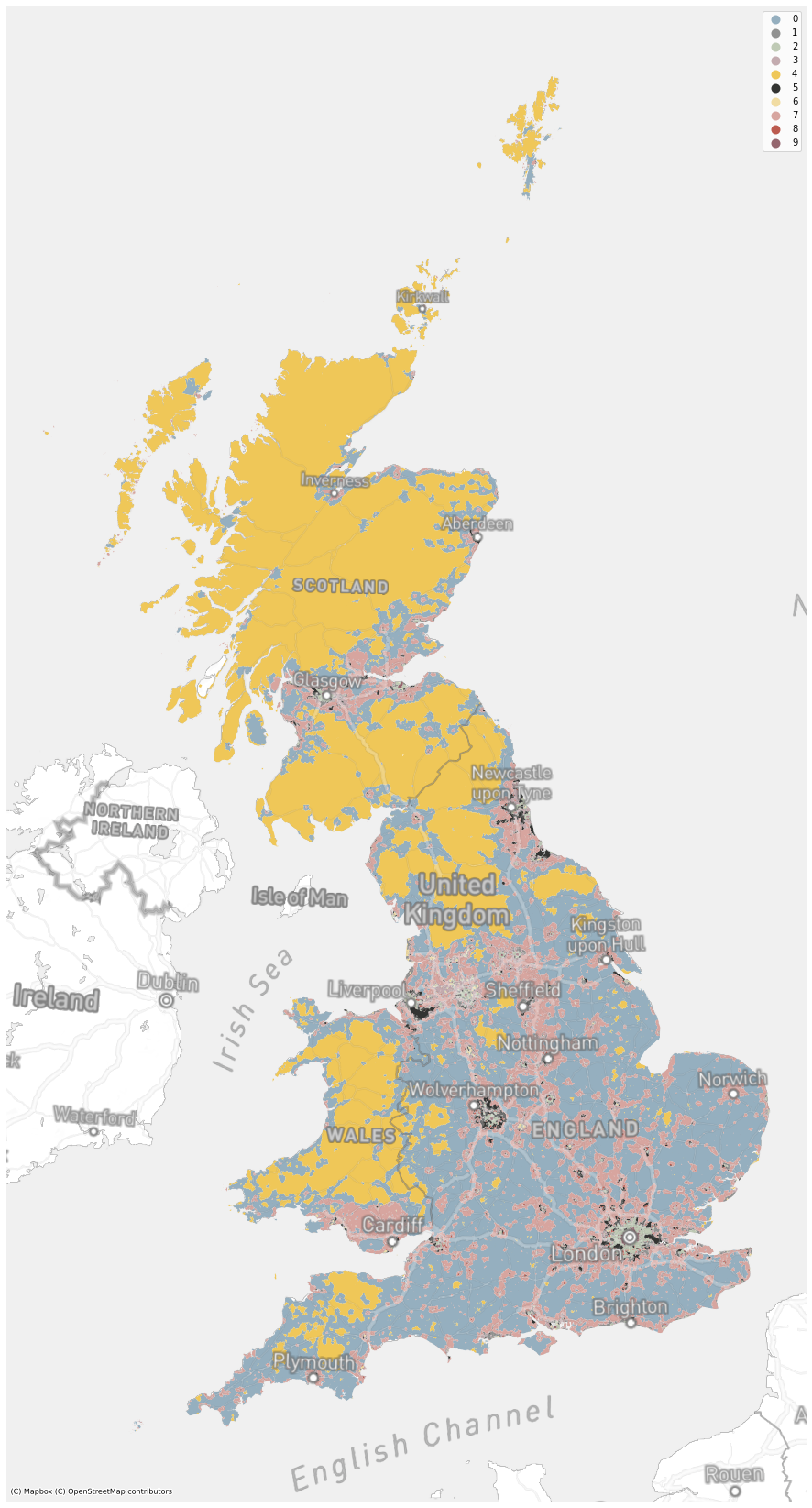
cmap = ugg.get_colormap(10, randomize=True)

token = ""

ax = spsig.plot("kmeans10gb", figsize=(20, 30), zorder=1, linewidth=0, edgecolor='w', alpha=1, legend=True, cmap=cmap, categorical=True)
ctx.add_basemap(ax, crs=27700, source=ugg.get_tiles('roads', token), zorder=2, alpha=.3)
ctx.add_basemap(ax, crs=27700, source=ugg.get_tiles('labels', token), zorder=3, alpha=1)
ctx.add_basemap(ax, crs=27700, source=ugg.get_tiles('background', token), zorder=-1, alpha=1)
ax.set_axis_off()

plt.savefig(f"../../urbangrammar_samba/spatial_signatures/signatures/signatures_KMeans10_GB.png")