Evaluation of the effect of chip size and origin¶

Compare performance of various models in relation to a chip size and origin (mosaic vs temporal)

import json
import glob

from itertools import product

import numpy
import pandas as pd
import matplotlib.pyplot as plt
import seaborn
import urbangrammar_graphics as ugg

path = "../../urbangrammar_samba/spatial_signatures/ai/gb_*_shuffled/json/"

results = glob.glob(path + "*")

names = [i[64:-5] + "_" + i[47:49] for i in results]

with open(results[0], "r") as f:
    result = json.load(f)

accuracy = pd.DataFrame(columns=["global"] + result["meta_class_names"], index=pd.MultiIndex.from_product([names, ["train", "val", "secret"]]))

for r in results[:-1]:
    with open(r, "r") as f:
        result = json.load(f)
    
    accuracy.loc[(result["model_name"]+ "_" + r[47:49], "train")] = [result["perf_model_accuracy_train"]] + result["perf_within_class_accuracy_train"]
    accuracy.loc[(result["model_name"]+ "_" + r[47:49], "val")] = [result["perf_model_accuracy_val"]] + result["perf_within_class_accuracy_val"]
    accuracy.loc[(result["model_name"]+ "_" + r[47:49], "secret")] = [result["perf_model_accuracy_secret"]] + result["perf_within_class_accuracy_secret"]

accuracy

		global	centres	periphery	Countryside agriculture	Wild countryside	Urban buffer
efficientnet_pooling_256_5_16	train	0.540909	0.716571	0.469743	0.500086	0.732914	0.285229
	val	0.532293	0.7104	0.4596	0.490533	0.728267	0.272667
	secret	0.537547	0.733733	0.453333	0.4912	0.730533	0.278933
efficientnet_pooling_256_5_64	train	0.825237	0.999681	0.978119	0.608968	0.857752	0.681666
	val	0.599028	0.876449	0.346168	0.480374	0.777009	0.51514
	secret	0.537702	0.698892	0.311963	0.46972	0.779252	0.511028
efficientnet_pooling_256_5_32	train	0.631566	0.912743	0.5622	0.5084	0.826914	0.347571
	val	0.561333	0.754533	0.4884	0.469467	0.796667	0.2976
	secret	0.561562	0.747511	0.494267	0.474133	0.800533	0.312933

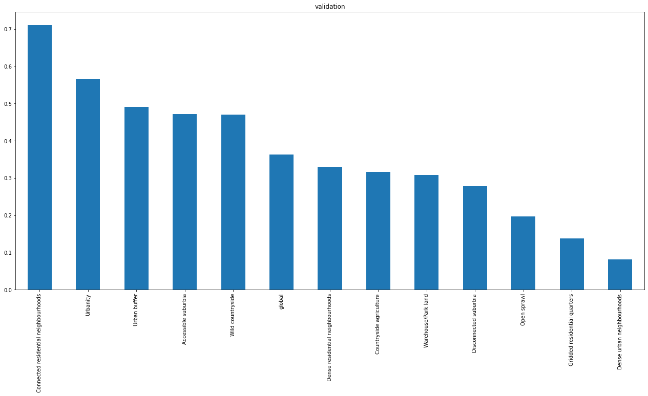
accuracy.xs('val', level=1).sort_index().plot.bar(figsize=(22, 10), title="validation")

<AxesSubplot:title={'center':'validation'}>

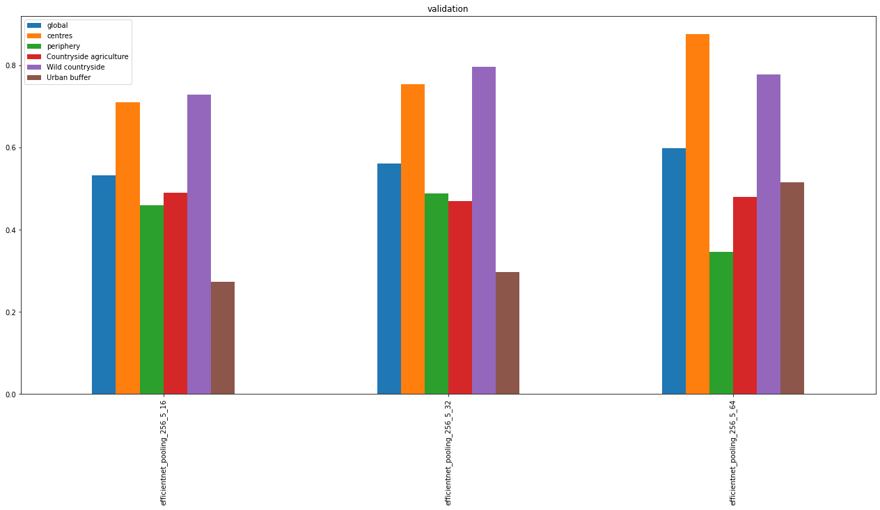
Notes:

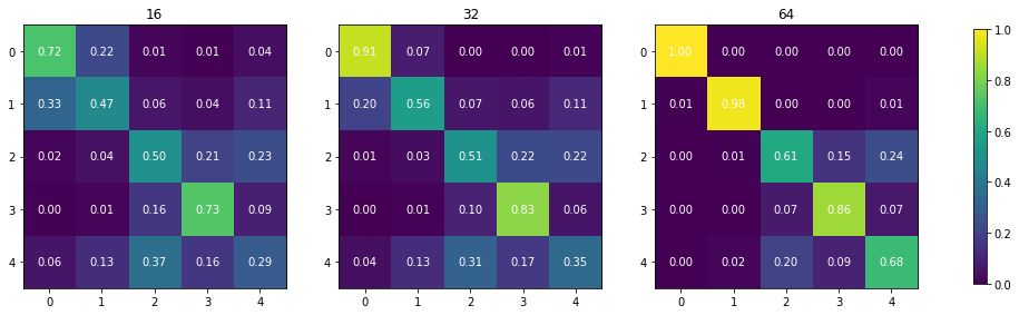
overall accuracy is unimpressive
in princple, larger chips have a better performance but there’s a big but - if you don’t do massive aggregation, you don’t have enough data for urban signature types
we’re not horrible in predicting centres and wild countryside
urban buffer is a challenging class due to the amout of greenery
periphery and countryside are somewhere in between
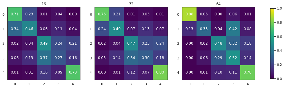
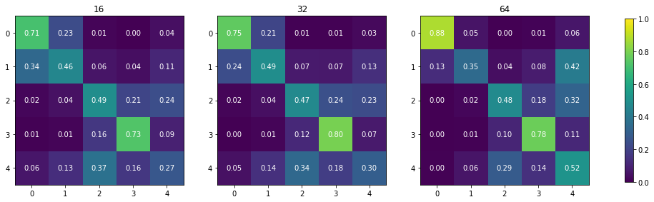
we’re good in predicting urban vs non-urban (two blocks on the confusion matrices)
we’re not putting urban buffer to countryside classes (conceptually) but the neural net is (empirically)
32 is empircally a better way of approximating signatures than 64 - when there is a space to fit 64x64 chip, it usually covers some adjacent green space because other signature types are too small to fit enough chips
- this could be mitigating by preferring chips with the larger number of intersections with underlying ET cells
  - count the number of intersections, sort and get N chips with the largest number. That way you limit the number of chips from large ET cells covering greenery.

ordered confusion matrix has a pattern similar to co-occurency matrix of singature types (empirical paper)

To-do:

prediction on 12 classes (combine only urbanity) and analyse the confusion matrix to know which to combine
we can try two parallel models, one with a single chip and another one with 3x3 chips around (or a few sampled) and merge before the end with a Dense to combine them [spatial lag]

Next steps:

prediction on 12 classes using 32x32 chips
- deirive aggregation
pipeline for John’s data to get way more chips
replicate 32x32 training with the new chips
- both 12 classes and aggregation
consider elimination of chips from large green ET cells (see note 8)
consider parallel model

Timeline:

Revisions by end of Feb
Empirical paper submitted by end of Apr
AI experiments by end of Apr
AI paper submitted by end of June

fig, axs = plt.subplots(1, 3, figsize=(18, 6))
for i, r in enumerate(sorted(results)):
    with open(r, "r") as f:
        result = json.load(f)
    a = numpy.array(result['perf_confusion_val'])
    a = a / a.sum(axis=1)[:, numpy.newaxis]
    a = pd.DataFrame(a).iloc[[0,1,2,4,3],[0,1,2,4,3]].values
    im = axs[i].imshow(a, cmap="viridis", vmin=0, vmax=1)
    for k, j in product(range(5), range(5)):
        axs[i].text(j, k, "{:.2f}".format(a[k, j]),
                       ha="center", va="center", color="w")
    axs[i].set_title(result['meta_chip_size'])
#     add labels
fig.colorbar(im, ax=axs[:], shrink=.7)

<matplotlib.colorbar.Colorbar at 0x7f5042555a30>

fig, axs = plt.subplots(1, 3, figsize=(18, 6))
for i, r in enumerate(sorted(results)):
    with open(r, "r") as f:
        result = json.load(f)
    a = numpy.array(result['perf_confusion_val'])
    a = a / a.sum(axis=1)[:, numpy.newaxis]
    im = axs[i].imshow(a, cmap="viridis", vmin=0, vmax=1)
    for k, j in product(range(5), range(5)):
        axs[i].text(j, k, "{:.2f}".format(a[k, j]),
                       ha="center", va="center", color="w")
    axs[i].set_title(result['meta_chip_size'])
fig.colorbar(im, ax=axs[:], shrink=.7)

<matplotlib.colorbar.Colorbar at 0x7f2dd8fd27f0>

fig, axs = plt.subplots(1, 3, figsize=(18, 6))
for i, r in enumerate(sorted(results)):
    with open(r, "r") as f:
        result = json.load(f)
    a = numpy.array(result['perf_confusion_train'])
    a = a / a.sum(axis=1)[:, numpy.newaxis]
    im = axs[i].imshow(a, cmap="viridis", vmin=0, vmax=1)
    for k, j in product(range(5), range(5)):
        axs[i].text(j, k, f"{a[k, j]:.2f}",
                       ha="center", va="center", color="w")
    axs[i].set_title(result['meta_chip_size'])
fig.colorbar(im, ax=axs[:], shrink=.7)

<matplotlib.colorbar.Colorbar at 0x7f2dd8d67e50>

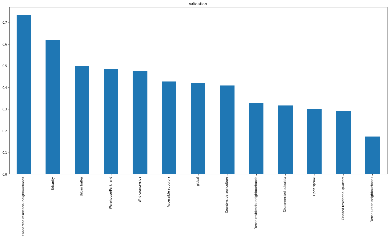
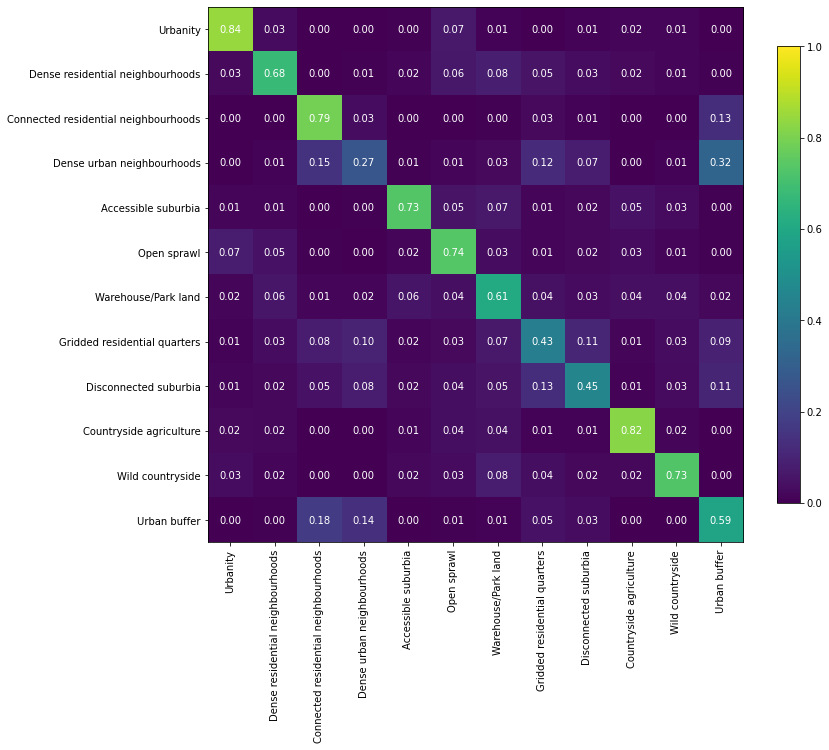
12 classes¶

results

['../../urbangrammar_samba/spatial_signatures/ai/gb_16_shuffled/json/efficientnet_pooling_256_5.json',
 '../../urbangrammar_samba/spatial_signatures/ai/gb_32_shuffled/json/efficientnet_pooling_256_12.json',
 '../../urbangrammar_samba/spatial_signatures/ai/gb_32_shuffled/json/efficientnet_pooling_256_5.json',
 '../../urbangrammar_samba/spatial_signatures/ai/gb_64_shuffled/json/efficientnet_pooling_256_5.json']

with open(results[1], "r") as f:
    result = json.load(f)

result["meta_class_names"] = [
        "Urbanity", 
        "Dense residential neighbourhoods",
        "Connected residential neighbourhoods",
        "Dense urban neighbourhoods",
        "Accessible suburbia",
        "Open sprawl",
        "Warehouse/Park land",
        "Gridded residential quarters",
        "Disconnected suburbia",
        "Countryside agriculture", 
        "Wild countryside", 
        "Urban buffer"
    ]

accuracy = pd.DataFrame(columns=["global"] + result["meta_class_names"], index=pd.Index(["train", "val", "secret"]))

accuracy.loc["train"] = [result["perf_model_accuracy_train"]] + result["perf_within_class_accuracy_train"]
accuracy.loc["val"] = [result["perf_model_accuracy_val"]] + result["perf_within_class_accuracy_val"]
accuracy.loc["secret"] = [result["perf_model_accuracy_secret"]] + result["perf_within_class_accuracy_secret"]

accuracy

	global	Urbanity	Dense residential neighbourhoods	Connected residential neighbourhoods	Dense urban neighbourhoods	Accessible suburbia	Open sprawl	Warehouse/Park land	Gridded residential quarters	Disconnected suburbia	Countryside agriculture	Wild countryside	Urban buffer
train	0.62358	0.844	0.677061	0.7896	0.2669	0.731106	0.7369	0.6127	0.4265	0.4537	0.822284	0.729964	0.5854
val	0.420283	0.618	0.328	0.7345	0.174	0.428009	0.302	0.4855	0.2905	0.3175	0.40856	0.476336	0.498
secret	0.428244	0.553905	0.28684	0.753	0.1915	0.384058	0.339	0.5035	0.285	0.327	0.608543	0.294023	0.5175

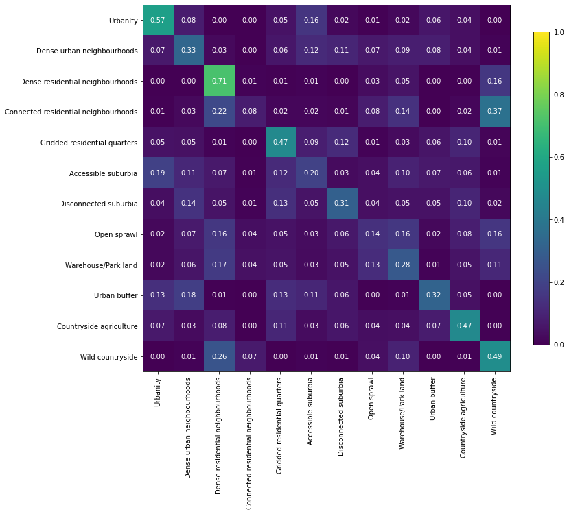
accuracy.loc['val'].sort_values(ascending=False).plot.bar(figsize=(22, 10), title="validation")

<AxesSubplot:title={'center':'validation'}>

a = numpy.array(result['perf_confusion_val'])
a = a / a.sum(axis=1)[:, numpy.newaxis]

order = numpy.array([0, 3, 1, 2, 7, 4, 8, 5, 6, 11, 9, 10], dtype=int)
a = pd.DataFrame(a).iloc[order, order].values

fig, ax = plt.subplots(figsize=(12, 12))


im = plt.imshow(a, cmap="viridis", vmin=0, vmax=1)
for k, j in product(range(12), range(12)):
    plt.text(j, k, "{:.2f}".format(a[k, j]),
                   ha="center", va="center", color="w")
fig.colorbar(im, ax=ax, shrink=.7)
plt.xticks(range(12),numpy.array(result["meta_class_names"])[order], rotation=90)
plt.yticks(range(12),numpy.array(result["meta_class_names"])[order])

([<matplotlib.axis.YTick at 0x7efc65b62610>,
  <matplotlib.axis.YTick at 0x7efc65b7ce20>,
  <matplotlib.axis.YTick at 0x7efc65b7c310>,
  <matplotlib.axis.YTick at 0x7efc70238820>,
  <matplotlib.axis.YTick at 0x7efc702f1700>,
  <matplotlib.axis.YTick at 0x7efc7023ee20>,
  <matplotlib.axis.YTick at 0x7efc702465b0>,
  <matplotlib.axis.YTick at 0x7efc70246d00>,
  <matplotlib.axis.YTick at 0x7efc7024a490>,
  <matplotlib.axis.YTick at 0x7efc7024abe0>,
  <matplotlib.axis.YTick at 0x7efc7024a3d0>,
  <matplotlib.axis.YTick at 0x7efc70246130>],
 [Text(0, 0, 'Urbanity'),
  Text(0, 1, 'Dense urban neighbourhoods'),
  Text(0, 2, 'Dense residential neighbourhoods'),
  Text(0, 3, 'Connected residential neighbourhoods'),
  Text(0, 4, 'Gridded residential quarters'),
  Text(0, 5, 'Accessible suburbia'),
  Text(0, 6, 'Disconnected suburbia'),
  Text(0, 7, 'Open sprawl'),
  Text(0, 8, 'Warehouse/Park land'),
  Text(0, 9, 'Urban buffer'),
  Text(0, 10, 'Countryside agriculture'),
  Text(0, 11, 'Wild countryside')])

fig, ax = plt.subplots(figsize=(12, 12))

a = numpy.array(result['perf_confusion_train'])
a = a / a.sum(axis=1)[:, numpy.newaxis]
im = plt.imshow(a, cmap="viridis", vmin=0, vmax=1)
for k, j in product(range(12), range(12)):
    plt.text(j, k, "{:.2f}".format(a[k, j]),
                   ha="center", va="center", color="w")
fig.colorbar(im, ax=ax, shrink=.7)
plt.xticks(range(12),result["meta_class_names"], rotation=90)
plt.yticks(range(12),result["meta_class_names"])

([<matplotlib.axis.YTick at 0x7fee9883fe80>,
  <matplotlib.axis.YTick at 0x7fee9883f760>,
  <matplotlib.axis.YTick at 0x7fee9886c850>,
  <matplotlib.axis.YTick at 0x7fee986f0220>,
  <matplotlib.axis.YTick at 0x7fee986f0970>,
  <matplotlib.axis.YTick at 0x7fee986f6100>,
  <matplotlib.axis.YTick at 0x7fee986f0940>,
  <matplotlib.axis.YTick at 0x7fee986e32e0>,
  <matplotlib.axis.YTick at 0x7fee986f60d0>,
  <matplotlib.axis.YTick at 0x7fee986f6c40>,
  <matplotlib.axis.YTick at 0x7fee986fc3d0>,
  <matplotlib.axis.YTick at 0x7fee986fcb20>],
 [Text(0, 0, 'Urbanity'),
  Text(0, 1, 'Dense residential neighbourhoods'),
  Text(0, 2, 'Connected residential neighbourhoods'),
  Text(0, 3, 'Dense urban neighbourhoods'),
  Text(0, 4, 'Accessible suburbia'),
  Text(0, 5, 'Open sprawl'),
  Text(0, 6, 'Warehouse/Park land'),
  Text(0, 7, 'Gridded residential quarters'),
  Text(0, 8, 'Disconnected suburbia'),
  Text(0, 9, 'Countryside agriculture'),
  Text(0, 10, 'Wild countryside'),
  Text(0, 11, 'Urban buffer')])

Temporal data¶

The same based on temporal chips

path = "../urbangrammar_samba/spatial_signatures/ai/gb_32_temporal/json/"

results = glob.glob(path + "*")

r = results[0]

with open(r, "r") as f:
    result = json.load(f)

accuracy = pd.DataFrame(columns=["global"] + result["meta_class_names"], index=pd.Index(["train", "val", "secret"]))

accuracy.loc["train"] = [result["perf_model_accuracy_train"]] + result["perf_within_class_accuracy_train"]
accuracy.loc["val"] = [result["perf_model_accuracy_val"]] + result["perf_within_class_accuracy_val"]
accuracy.loc["secret"] = [result["perf_model_accuracy_secret"]] + result["perf_within_class_accuracy_secret"]

accuracy.loc['val'].sort_values(ascending=False).plot.bar(figsize=(22, 10), title="validation")

<AxesSubplot:title={'center':'validation'}>

a = numpy.array(result['perf_confusion_val'])
a = a / a.sum(axis=1)[:, numpy.newaxis]

# order = numpy.array([0, 3, 1, 2, 7, 4, 8, 5, 6, 11, 9, 10], dtype=int)
# a = pd.DataFrame(a).iloc[order, order].values

fig, ax = plt.subplots(figsize=(12, 12))


im = plt.imshow(a, cmap="viridis", vmin=0, vmax=1)
for k, j in product(range(12), range(12)):
    plt.text(j, k, "{:.2f}".format(a[k, j]),
                   ha="center", va="center", color="w")
fig.colorbar(im, ax=ax, shrink=.7)
plt.xticks(range(12),numpy.array(result["meta_class_names"])[order], rotation=90)
plt.yticks(range(12),numpy.array(result["meta_class_names"])[order])

([<matplotlib.axis.YTick at 0x7f9ac06168b0>,
  <matplotlib.axis.YTick at 0x7f9ac0616130>,
  <matplotlib.axis.YTick at 0x7f9ac064fa90>,
  <matplotlib.axis.YTick at 0x7f9ac0421ac0>,
  <matplotlib.axis.YTick at 0x7f9ac04986d0>,
  <matplotlib.axis.YTick at 0x7f9ac042b340>,
  <matplotlib.axis.YTick at 0x7f9ac042bac0>,
  <matplotlib.axis.YTick at 0x7f9ac0434250>,
  <matplotlib.axis.YTick at 0x7f9ac04349a0>,
  <matplotlib.axis.YTick at 0x7f9ac0434850>,
  <matplotlib.axis.YTick at 0x7f9ac042b4f0>,
  <matplotlib.axis.YTick at 0x7f9ac0427790>],
 [Text(0, 0, 'Urbanity'),
  Text(0, 1, 'Dense urban neighbourhoods'),
  Text(0, 2, 'Dense residential neighbourhoods'),
  Text(0, 3, 'Connected residential neighbourhoods'),
  Text(0, 4, 'Gridded residential quarters'),
  Text(0, 5, 'Accessible suburbia'),
  Text(0, 6, 'Disconnected suburbia'),
  Text(0, 7, 'Open sprawl'),
  Text(0, 8, 'Warehouse/Park land'),
  Text(0, 9, 'Urban buffer'),
  Text(0, 10, 'Countryside agriculture'),
  Text(0, 11, 'Wild countryside')])

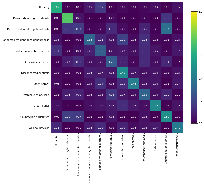
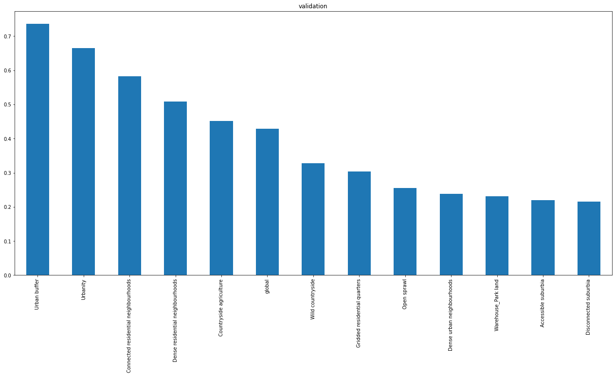
Balanced data¶

path = "../../urbangrammar_samba/spatial_signatures/ai/gb_32_balanced_named_v2/json/"

results = glob.glob(path + "*")

r = results[0]

with open(r, "r") as f:
    result = json.load(f)

accuracy = pd.DataFrame(columns=["global"] + result["meta_class_names"], index=pd.Index(["train", "val", "secret"]))

accuracy.loc["train"] = [result["perf_model_accuracy_train"]] + result["perf_within_class_accuracy_train"]
accuracy.loc["val"] = [result["perf_model_accuracy_val"]] + result["perf_within_class_accuracy_val"]
accuracy.loc["secret"] = [result["perf_model_accuracy_secret"]] + result["perf_within_class_accuracy_secret"]

accuracy

	global	Urbanity	Dense residential neighbourhoods	Connected residential neighbourhoods	Dense urban neighbourhoods	Accessible suburbia	Open sprawl	Warehouse_Park land	Gridded residential quarters	Disconnected suburbia	Countryside agriculture	Wild countryside	Urban buffer
train	0.554045	0.769971	0.707678	0.615457	0.538372	0.600216	0.477016	0.589415	0.393829	0.233229	0.683429	0.462629	0.762229
val	0.428392	0.6646	0.507874	0.5828	0.238587	0.219465	0.254962	0.230869	0.304	0.2158	0.452206	0.3276	0.7366
secret	0.439124	0.6722	0.481884	0.5816	0.237983	0.211743	0.163166	0.377451	0.286	0.2152	0.383388	0.3482	0.7412

accuracy.loc['val'].sort_values(ascending=False).plot.bar(figsize=(22, 10), title="validation")

<AxesSubplot:title={'center':'validation'}>

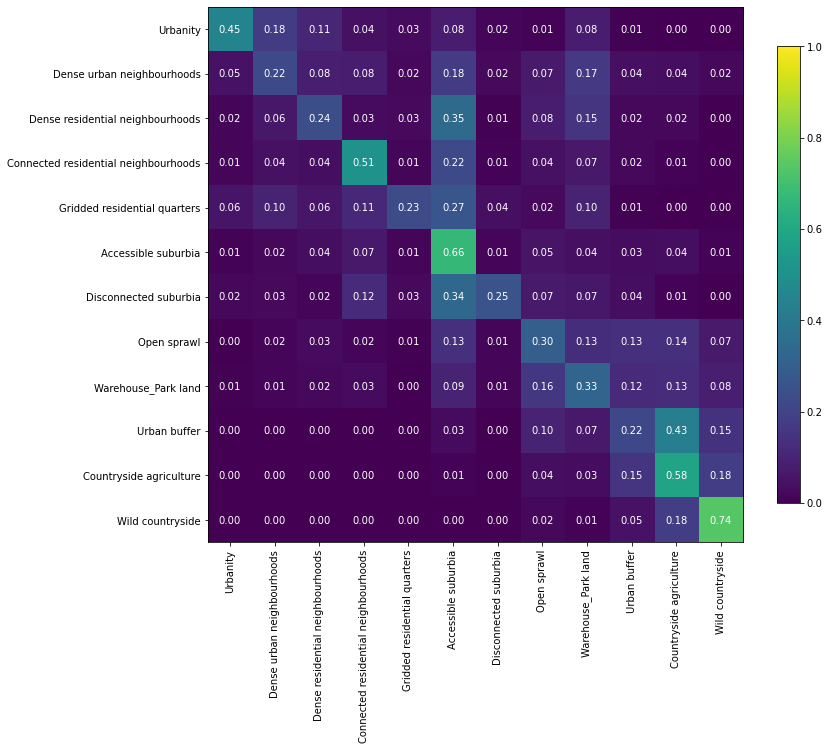
a = numpy.array(result['perf_confusion_val'])
a = a / a.sum(axis=1)[:, numpy.newaxis]

order = numpy.array([9, 4, 3, 1, 6, 0, 5, 7, 10, 8, 2, 11], dtype=int)
a = pd.DataFrame(a).iloc[order, order].values

fig, ax = plt.subplots(figsize=(12, 12))


im = plt.imshow(a, vmin=0, vmax=1, cmap='viridis')
for k, j in product(range(12), range(12)):
    plt.text(j, k, "{:.2f}".format(a[k, j]),
                   ha="center", va="center", color="w")
fig.colorbar(im, ax=ax, shrink=.7)
ticks = numpy.array(sorted(result["meta_class_names"]))[order]
plt.xticks(range(12),ticks, rotation=90)
plt.yticks(range(12),ticks)
plt.savefig("figs/image_class_conf.pdf")

Urban Grammar AI | WP3 - Signature AI

Evaluation of the effect of chip size and origin¶

12 classes¶

Temporal data¶

Balanced data¶