This capsule1 considers the make up of green belt areas in England using the Spatial Signatures (Fleischmann and Arribas-Bel 2022). You can see more on the data used, and how they have been combined, in the Data Aquisition section. We reserve this document to present the main results.
1
Code
import warningswarnings.filterwarnings("ignore")import pandasimport geopandasimport jsonimport requestsimport contextilyimport xyzservicesimport matplotlib.pyplot as pltimport matplotlib.patches as mpatchesfrom matplotlib.colors import to_heximport urbangrammar_graphics as uggdef build_tab(db): areas = ( db .assign(area=db.area/1e6) .groupby('type') ['area'] .sum() .sort_values(ascending=False) ) tab = pandas.DataFrame( {'Area (Sq.Km)': areas, '% of total area': areas *100/ areas.sum()} )return tab.round(2)def build_plot(tab, label=None, context=None, figsize=(2, 6)): ttp = tab['% of total area'].sort_values() ax = ttp.plot.barh( color='k', figsize=figsize, title='% of area by signature', label=label )if context isnotNone: ( context ['% of total area'] .reindex(ttp.index) .plot.barh( edgecolor='#8fa37e', facecolor='none', linewidth=2, ax=ax, label='National' ) ) ax.set_axis_off()if (label isnotNone) and (context isnotNone): plt.legend(loc='lower right', frameon=False)return axdef get_signature_colors(name=True):""" Ported from here as unreleased: https://github.com/urbangrammarai/graphics/blob/69bf5976a11c783fc8a27f59ef57efefbbee6aa8/urbangrammar_graphics/graphics.py#L207-L272 Get a dictionary of colors mapped to signatures classes of Great Britain Parameters ---------- name : bool `True` maps to names, `False` maps to string keys (e.g. `'2_1'`) Returns ------- dict """ cols = ugg.get_colormap(20, randomize=False).colors key = {"0_0": cols[16],"1_0": cols[15],"3_0": cols[9],"4_0": cols[12],"5_0": cols[21],"6_0": cols[8],"7_0": cols[4],"8_0": cols[18],"2_0": cols[6],"2_1": cols[23],"2_2": cols[19],"9_0": cols[7],"9_1": cols[3],"9_2": cols[22],"9_3": cols[0], # outlier"9_4": cols[11],"9_5": cols[14],"9_6": cols[0], # outlier"9_7": cols[0], # outlier"9_8": cols[0], # outlier }if name: types = {"0_0": "Countryside agriculture","1_0": "Accessible suburbia","3_0": "Open sprawl","4_0": "Wild countryside","5_0": "Warehouse/Park land","6_0": "Gridded residential quarters","7_0": "Urban buffer","8_0": "Disconnected suburbia","2_0": "Dense residential neighbourhoods","2_1": "Connected residential neighbourhoods","2_2": "Dense urban neighbourhoods","9_0": "Local urbanity","9_1": "Concentrated urbanity","9_2": "Regional urbanity","9_4": "Metropolitan urbanity","9_5": "Hyper concentrated urbanity","9_3": "outlier","9_6": "outlier","9_7": "outlier","9_8": "outlier", }return {v: key[k] for k, v in types.items()}return keysig_colors = get_signature_colors()def build_legend(types, sig_colors=sig_colors): ps = []for t in types: type_patch = mpatches.Patch(color=sig_colors[t], label=t) ps.append(type_patch)return psdb = geopandas.read_parquet('ss_clipped.pq')
National statistics
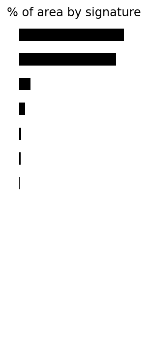
We begin with a table that summarises the form and function makeup of English green belts. To do this, we show the total area and the proportion of the total green belt land that is occupied by each of the 16 signature types.2
The most common class, “Urban buffer”, is hardly a surprise since the notion of green belt is worked into its very definition. From the original signature descriptions3, Urban buffer is:
“Urban buffer” can be characterised as a green belt around cities. This signature includes mostly agricultural land in the immediate adjacency of towns and cities, often including edge development. It still feels more like countryside than urban, but these signatures are much smaller compared to other countryside types.
However, less than half of green belts are classified as “Urban buffer”. The rest is a combination of other classes, including “Countryside agriculture” (>40%), and “Open Sprawl” (>5%), as well as a long tail of other signatures with smaller contributions. To help the reader get a sense of what these classes represent, we include here the definitions (pen portraits) of the two most relevant ones:
Countryside agriculture
“Countryside agriculture” features much of the English countryside and displays a high degree of agriculture including both fields and pastures. There are a few buildings scattered across the area but, for the most part, it is green space.
Open Sprawl
“Open sprawl” represents the transition between countryside and urbanised land. It is located in the outskirts of cities or around smaller towns and is typically made up of large open space areas intertwined with different kinds of human development, from highways to smaller neighbourhoods.
The reader can refer to this additional document for descriptions of all the classes:
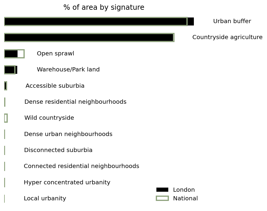
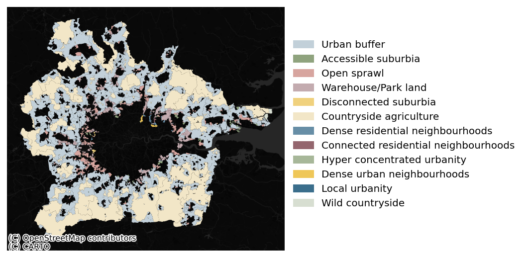
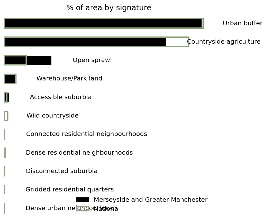
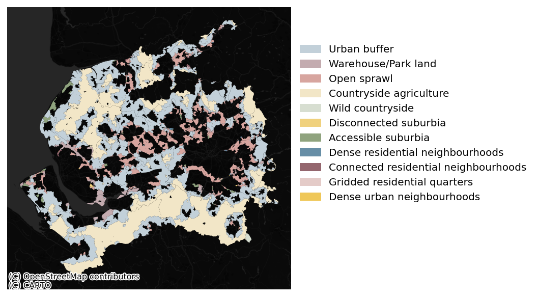
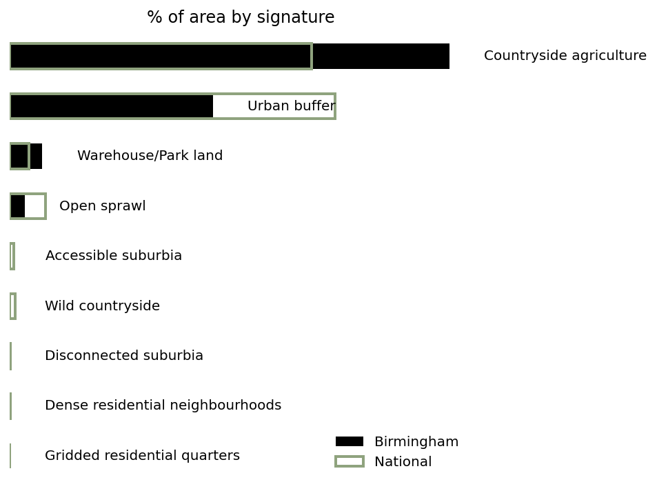
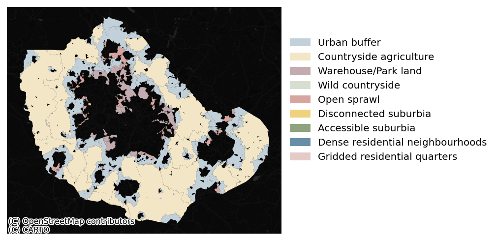
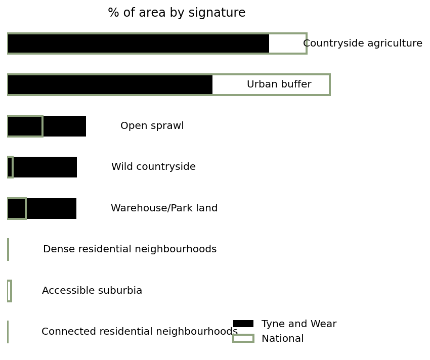
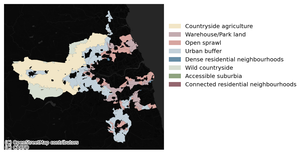
The proportions above are national aggregates, and it is possible that the signature mix varies across different urban areas. To explore this, below we present maps to explore five English cities.
Fleischmann, Martin, and Daniel Arribas-Bel. 2022. “Geographical Characterisation of British Urban Form and Function Using the Spatial Signatures Framework.”Scientific Data 9 (1): 1–15.